Feature summary
feature_summary.RmdCreate Metaboprep object
library(metaboprep)

# import data
data     <- read.csv(system.file("extdata", "dummy_data.csv",     package = "metaboprep"), header=T, row.names = 1) |> as.matrix()
samples  <- read.csv(system.file("extdata", "dummy_samples.csv",  package = "metaboprep"), header=T, row.names = 1)
features <- read.csv(system.file("extdata", "dummy_features.csv", package = "metaboprep"), header=T, row.names = 1)

# create object
mydata <- Metaboprep(data = data, samples = samples, features = features)
Summary of Metaboprep object
summary(mydata)
#> Metaboprep Object Summary
#> --------------------------
#> Samples      : 100
#> Features     : 20
#> Data Layers  : 1
#> Layer Names  : input
#>
#> Sample Summary Layers : none
#> Feature Summary Layers: none
#>
#> Sample Annotation (metadata):
#>   Columns: 5
#>   Names  : sample_id, age, sex, pos, neg
#>
#> Feature Annotation (metadata):
#>   Columns: 5
#>   Names  : feature_id, platform, pathway, derived_feature, xenobiotic_feature
#>
#> Exclusion Codes Summary:
#>
#>   Sample Exclusions:
#> Exclusion | Count
#> -----------------
#> user_excluded                     | 0
#> extreme_sample_missingness        | 0
#> user_defined_sample_missingness   | 0
#> user_defined_sample_totalpeakarea | 0
#> user_defined_sample_pca_outlier   | 0
#>
#>   Feature Exclusions:
#> Exclusion | Count
#> -----------------
#> user_excluded                    | 0
#> extreme_feature_missingness      | 0
#> user_defined_feature_missingness | 0
Run feature summary
# note that for illustrative purposes we are using a log outlier unit distance of 1.0 here, in practice we tend to favor a value of 5.0.
feature_sum1 <- feature_summary(metaboprep     = mydata,
                                source_layer    = "input",
                                outlier_udist   = 1.0,
                                tree_cut_height = 0.5,
                                output          = "data.frame",
                                cores           = 1)
Table of feature summary
| feature_id | missingness | outlier_count | n | mean | sd | median | min | max | range | skew | kurtosis | se | missing | var | disp_index | coef_variance | W | log10_W | k | independent_features |
|---|---|---|---|---|---|---|---|---|---|---|---|---|---|---|---|---|---|---|---|---|
| metab_id_1 | 0 | 5 | 100 | 0.511 | 0.293 | 0.530 | 0.000 | 0.993 | 0.992 | -0.123 | -1.231 | 0.029 | 0 | 0.086 | 0.168 | 0.574 | 0.949 | 0.744 | 1 | TRUE |
| metab_id_2 | 0 | 0 | 100 | 0.521 | 0.310 | 0.547 | 0.018 | 0.993 | 0.975 | -0.150 | -1.404 | 0.031 | 0 | 0.096 | 0.184 | 0.594 | 0.924 | 0.834 | 2 | TRUE |
| metab_id_3 | 0 | 10 | 100 | 0.488 | 0.283 | 0.504 | 0.001 | 0.995 | 0.994 | -0.036 | -1.109 | 0.028 | 0 | 0.080 | 0.165 | 0.580 | 0.963 | 0.749 | 3 | TRUE |
| metab_id_4 | 0 | 5 | 100 | 0.464 | 0.286 | 0.466 | 0.004 | 0.992 | 0.988 | 0.092 | -1.199 | 0.029 | 0 | 0.082 | 0.177 | 0.617 | 0.954 | 0.833 | 4 | TRUE |
| metab_id_5 | 0 | 11 | 100 | 0.521 | 0.293 | 0.547 | 0.004 | 0.976 | 0.972 | -0.219 | -1.161 | 0.029 | 0 | 0.086 | 0.164 | 0.561 | 0.945 | 0.782 | 5 | TRUE |
| metab_id_6 | 0 | 7 | 100 | 0.490 | 0.259 | 0.473 | 0.007 | 0.993 | 0.986 | 0.007 | -1.006 | 0.026 | 0 | 0.067 | 0.137 | 0.528 | 0.973 | 0.803 | 6 | TRUE |
| metab_id_7 | 0 | 7 | 100 | 0.479 | 0.277 | 0.441 | 0.029 | 0.992 | 0.963 | 0.135 | -1.211 | 0.028 | 0 | 0.077 | 0.160 | 0.579 | 0.953 | 0.899 | 7 | TRUE |
| metab_id_8 | 0 | 0 | 100 | 0.476 | 0.312 | 0.491 | 0.001 | 0.999 | 0.998 | 0.059 | -1.350 | 0.031 | 0 | 0.097 | 0.205 | 0.656 | 0.936 | 0.796 | 8 | TRUE |
| metab_id_9 | 0 | 10 | 100 | 0.468 | 0.260 | 0.489 | 0.005 | 0.975 | 0.971 | 0.000 | -1.090 | 0.026 | 0 | 0.068 | 0.144 | 0.556 | 0.968 | 0.800 | 9 | TRUE |
| metab_id_10 | 0 | 0 | 100 | 0.524 | 0.290 | 0.532 | 0.019 | 0.993 | 0.974 | -0.158 | -1.252 | 0.029 | 0 | 0.084 | 0.161 | 0.554 | 0.945 | 0.841 | 10 | TRUE |
Feature summary attributes
In addition to the summary data, the hierarchical cluster dendrogram
is appended to the returned data.frame as and
attribute. This can be accessed with the attribute name:
[source_layer]_tree, in this case we summarised the
input data, therefore the attribute name is
input_tree.
suppressPackageStartupMessages(library(dendextend))

# extract tree from attributes
tree <- attr(feature_sum1, 'input_tree')
dend <- stats::as.dendrogram(tree)

# color the independent features blue
metab_color       <- feature_sum1[, c("feature_id", "independent_features")]
metab_color       <- metab_color[match(labels(dend), metab_color$feature_id), ]
metab_color$color <- ifelse(metab_color$independent_features==TRUE, "#477EB8", "grey")

# format dendrogram for ploting
dend <- dend |>
  dendextend::set("labels_cex", 0.75) |>
  dendextend::set("labels_col", metab_color$color) |>
  dendextend::set("branches_lwd", 1) |>
  dendextend::set("branches_k_color",  value = metab_color$color)

## plot the dendrogram
dend |> plot(main = "Feature clustering dendrogram")
abline(h = 0.5, col = "#E41A1C", lwd = 1.5)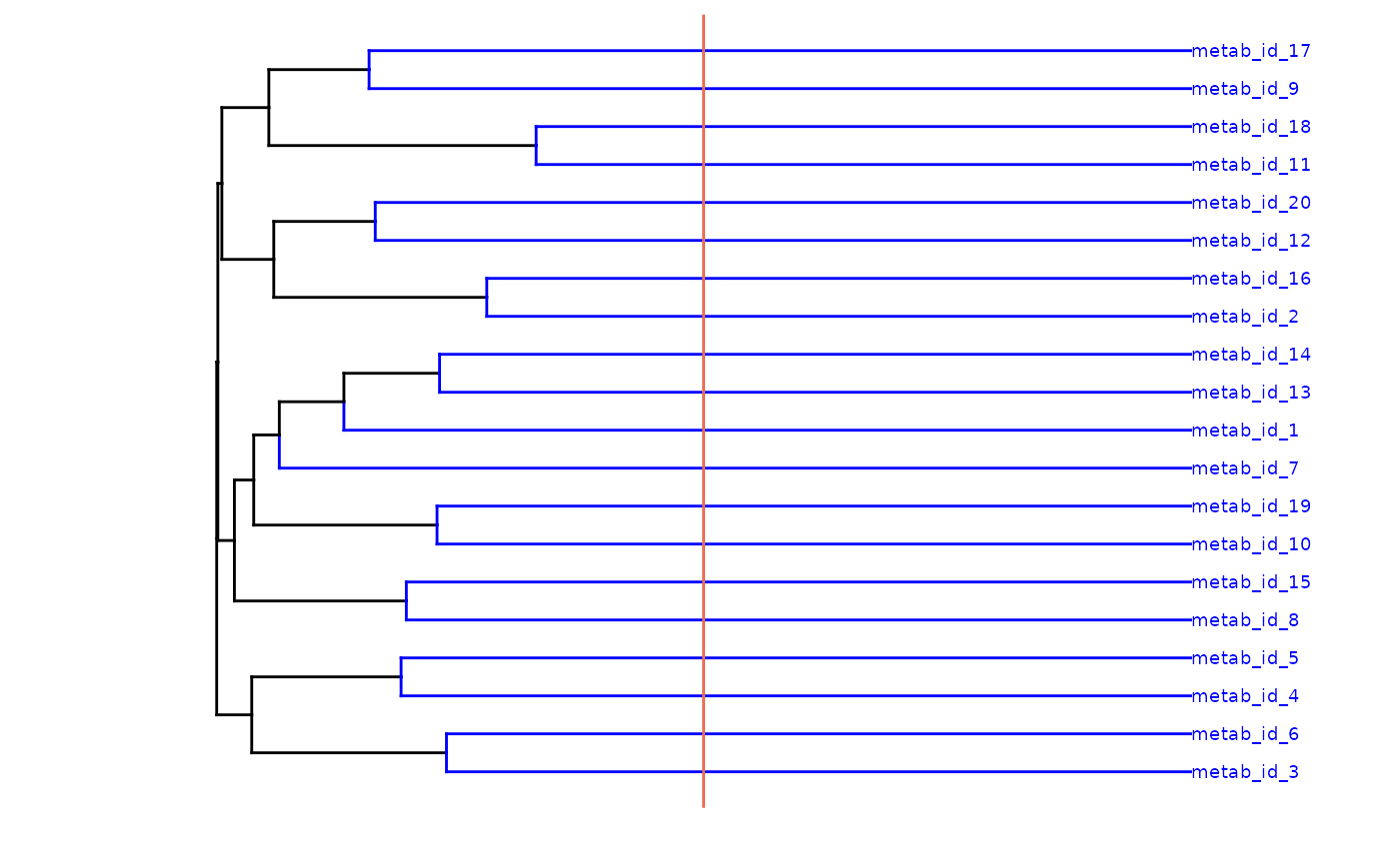
Run feature summary on subset
Using the sample_ids and feature_ids
arguments you can run the summary for a subset of the data. Note: all
rows will be return, however summary data will only be returned for the
specified ids.
## define a vector of sample IDs
sids <- mydata@samples[mydata@samples$sex == "female", "sample_id"]

## define a vector of feature IDs
fids <- mydata@features[, "feature_id"] |> sample(10)

# note that for illustrative purposes we are using a log outlier unit distance of 1.0 here, in practice we tend to favor a value of 5.0.
feature_sum_subset <- feature_summary(metaboprep      = mydata,
                                      source_layer    = "input",
                                      outlier_udist   = 1.0,
                                      tree_cut_height = 0.5,
                                      sample_ids      = sids,
                                      feature_ids     = fids,
                                      output          = "data.frame",
                                      cores           = 1)
Table of feature summary for subset
| feature_id | missingness | outlier_count | n | mean | sd | median | min | max | range | skew | kurtosis | se | missing | var | disp_index | coef_variance | W | log10_W | k | independent_features |
|---|---|---|---|---|---|---|---|---|---|---|---|---|---|---|---|---|---|---|---|---|
| metab_id_4 | 0 | 5 | 55 | 0.498 | 0.273 | 0.478 | 0.009 | 0.992 | 0.983 | 0.094 | -1.159 | 0.037 | 0 | 0.075 | 0.150 | 0.549 | 0.960 | 0.836 | 7 | TRUE |
| metab_id_5 | 0 | 9 | 55 | 0.580 | 0.296 | 0.632 | 0.013 | 0.976 | 0.963 | -0.436 | -1.035 | 0.040 | 0 | 0.087 | 0.151 | 0.510 | 0.929 | 0.734 | 3 | TRUE |
| metab_id_6 | 0 | 6 | 55 | 0.520 | 0.284 | 0.560 | 0.007 | 0.993 | 0.986 | -0.273 | -1.103 | 0.038 | 0 | 0.080 | 0.155 | 0.546 | 0.952 | 0.757 | 4 | TRUE |
| metab_id_9 | 0 | 6 | 55 | 0.461 | 0.270 | 0.489 | 0.005 | 0.975 | 0.971 | 0.012 | -1.151 | 0.036 | 0 | 0.073 | 0.158 | 0.585 | 0.963 | 0.798 | 9 | TRUE |
| metab_id_12 | 0 | 0 | 55 | 0.518 | 0.296 | 0.498 | 0.006 | 0.989 | 0.983 | -0.125 | -1.233 | 0.040 | 0 | 0.088 | 0.170 | 0.573 | 0.946 | 0.801 | 2 | TRUE |
| metab_id_13 | 0 | 4 | 55 | 0.544 | 0.313 | 0.595 | 0.005 | 0.990 | 0.984 | -0.265 | -1.325 | 0.042 | 0 | 0.098 | 0.181 | 0.576 | 0.927 | 0.752 | 1 | TRUE |
| metab_id_15 | 0 | 7 | 55 | 0.495 | 0.280 | 0.522 | 0.032 | 0.991 | 0.959 | 0.054 | -1.139 | 0.038 | 0 | 0.078 | 0.158 | 0.566 | 0.961 | 0.874 | 5 | TRUE |
| metab_id_16 | 0 | 3 | 55 | 0.463 | 0.315 | 0.447 | 0.005 | 0.998 | 0.992 | 0.276 | -1.384 | 0.042 | 0 | 0.099 | 0.214 | 0.679 | 0.909 | 0.868 | 6 | TRUE |
| metab_id_17 | 0 | 3 | 55 | 0.449 | 0.287 | 0.437 | 0.025 | 0.972 | 0.947 | 0.185 | -1.280 | 0.039 | 0 | 0.083 | 0.184 | 0.639 | 0.938 | 0.902 | 8 | TRUE |
| metab_id_18 | 0 | 1 | 55 | 0.536 | 0.316 | 0.599 | 0.028 | 0.999 | 0.971 | -0.073 | -1.480 | 0.043 | 0 | 0.100 | 0.186 | 0.590 | 0.918 | 0.867 | 10 | TRUE |
Run sample & feature summaries together
# note that for illustrative purposes we are using a log outlier unit distance of 1.0 here, in practice we tend to favor a value of 5.0.
sam_n_feat_sum <- summarise(metaboprep      = mydata,
                            source_layer    = "input",
                            outlier_udist   = 1.0,
                            tree_cut_height = 0.5,
                            sample_ids      = sids,
                            feature_ids     = fids,
                            output          = "data.frame",
                            cores           = 1)
#> AF =  1
Table of feature summary for subset
| feature_id | missingness | outlier_count | n | mean | sd | median | min | max | range | skew | kurtosis | se | missing | var | disp_index | coef_variance | W | log10_W | k | independent_features |
|---|---|---|---|---|---|---|---|---|---|---|---|---|---|---|---|---|---|---|---|---|
| metab_id_4 | 0 | 5 | 55 | 0.498 | 0.273 | 0.478 | 0.009 | 0.992 | 0.983 | 0.094 | -1.159 | 0.037 | 0 | 0.075 | 0.150 | 0.549 | 0.960 | 0.836 | 7 | TRUE |
| metab_id_5 | 0 | 9 | 55 | 0.580 | 0.296 | 0.632 | 0.013 | 0.976 | 0.963 | -0.436 | -1.035 | 0.040 | 0 | 0.087 | 0.151 | 0.510 | 0.929 | 0.734 | 3 | TRUE |
| metab_id_6 | 0 | 6 | 55 | 0.520 | 0.284 | 0.560 | 0.007 | 0.993 | 0.986 | -0.273 | -1.103 | 0.038 | 0 | 0.080 | 0.155 | 0.546 | 0.952 | 0.757 | 4 | TRUE |
| metab_id_9 | 0 | 6 | 55 | 0.461 | 0.270 | 0.489 | 0.005 | 0.975 | 0.971 | 0.012 | -1.151 | 0.036 | 0 | 0.073 | 0.158 | 0.585 | 0.963 | 0.798 | 9 | TRUE |
| metab_id_12 | 0 | 0 | 55 | 0.518 | 0.296 | 0.498 | 0.006 | 0.989 | 0.983 | -0.125 | -1.233 | 0.040 | 0 | 0.088 | 0.170 | 0.573 | 0.946 | 0.801 | 2 | TRUE |
| metab_id_13 | 0 | 4 | 55 | 0.544 | 0.313 | 0.595 | 0.005 | 0.990 | 0.984 | -0.265 | -1.325 | 0.042 | 0 | 0.098 | 0.181 | 0.576 | 0.927 | 0.752 | 1 | TRUE |
| metab_id_15 | 0 | 7 | 55 | 0.495 | 0.280 | 0.522 | 0.032 | 0.991 | 0.959 | 0.054 | -1.139 | 0.038 | 0 | 0.078 | 0.158 | 0.566 | 0.961 | 0.874 | 5 | TRUE |
| metab_id_16 | 0 | 3 | 55 | 0.463 | 0.315 | 0.447 | 0.005 | 0.998 | 0.992 | 0.276 | -1.384 | 0.042 | 0 | 0.099 | 0.214 | 0.679 | 0.909 | 0.868 | 6 | TRUE |
| metab_id_17 | 0 | 3 | 55 | 0.449 | 0.287 | 0.437 | 0.025 | 0.972 | 0.947 | 0.185 | -1.280 | 0.039 | 0 | 0.083 | 0.184 | 0.639 | 0.938 | 0.902 | 8 | TRUE |
| metab_id_18 | 0 | 1 | 55 | 0.536 | 0.316 | 0.599 | 0.028 | 0.999 | 0.971 | -0.073 | -1.480 | 0.043 | 0 | 0.100 | 0.186 | 0.590 | 0.918 | 0.867 | 10 | TRUE |