Using gpmapr

library(gpmapr)

Introduction

The gpmapr package provides a set of functions to interact with the GPMap API.

Getting started

The first port of entry is the search_gpmap function. This function allows you to search for a trait, gene, or variant.

haemoglobin <- search_gpmap("haemoglobin")
knitr::kable(haemoglobin[, c("name", "sample_size", "num_coloc_groups", "call")])

	name	sample_size	num_coloc_groups	call
43431	Glycated haemoglobin levels	146806	93	trait(915)
43436	Haemoglobin concentration	563946	828	trait(920)
43438	Mean corpuscular haemoglobin concentration	491553	297	trait(922)
43447	Haemoglobin	408112	757	trait(931)
44152	Haemoglobin levels	445373	775	trait(1636)
44156	Haemoglobin A1c levels	437749	838	trait(1640)
44499	Mean corpuscular haemoglobin	572863	936	trait(1983)
45100	Haemoglobin concentration (UKB data field 30020)	396624	658	trait(2584)
45127	Glycated haemoglobin HbA1c levels (UKB data field 30750)	389889	721	trait(2611)
47275	Haemoglobin concentration	350474	497	trait(4759)
47277	Mean corpuscular haemoglobin	350472	628	trait(4761)
47278	Mean corpuscular haemoglobin concentration	350468	137	trait(4762)
52158	Mean corpuscular haemoglobin	430998	628	trait(4761)
52788	Mean corpuscular haemoglobin concentration	430998	137	trait(4762)
53046	Glycated haemoglobin HbA1c (30750)	430998	0	trait(42778)
53057	Haemoglobin concentration	430998	497	trait(4759)

You can see information about the different traits that match your search, how to subsequently get more information (under call), and metadata about the trait (under info).

Understanding info

• Extractions: Each trait has a number of extractions, related to the number of finemapped ld regions that had a p-value < 1.5e-4.
• Colocalisation Groups: The number of colocalisation groups associated with the trait / gene / variant.
• Colocalising Traits: The number of traits that are colocalising with the trait / gene / variant.
• Rare Result Groups: Each trait has a number of rare result groups, related to the number of groups of rare result groups that had a p-value < 1.5e-4.

You can also search for a gene (by ENSG ID or gene name) or variant (by CHR:BP or rsID).

knitr::kable(search_gpmap("SLC44A")[, c("name", "sample_size", "num_study_extractions", "num_coloc_groups", "call")])

	name	sample_size	num_study_extractions	num_coloc_groups	call
1032	SLC44A1 (ENSG00000070214)	NA	206	9	gene(‘SLC44A1’)
5825	SLC44A2 (ENSG00000129353)	NA	226	14	gene(‘SLC44A2’)
7196	SLC44A5 (ENSG00000137968)	NA	91	9	gene(‘SLC44A5’)
7921	SLC44A3 (ENSG00000143036)	NA	361	17	gene(‘SLC44A3’)
17220	SLC44A4 (ENSG00000204385)	NA	107	12	gene(‘SLC44A4’)
19708	SLC44A3-AS1 (ENSG00000224081)	NA	179	12	gene(‘SLC44A3-AS1’)

knitr::kable(search_gpmap("22:37042914"))

type	name	type_id	num_coloc_groups	num_coloc_studies	num_rare_results	num_study_extractions	call
original_variant	22:37042914 T/C	5521294	0	0	0	NA	variant(5521294)

Variant search returns proxy variants

The variant search will return the original variant and any proxy variants that are in LD with the original variant, which also have colocalisation results. Each variant is marked as either original_variant or proxy_variant. In this example, the original variant has no colocalisation results, but the proxy variant does. The proxy variant is also marked as having a r^2 of 0.96

proxy_variants <- search_gpmap("rs17078078")
knitr::kable(proxy_variants)

type	name	type_id	num_coloc_groups	num_coloc_studies	num_rare_results	num_study_extractions	call
original_variant	3:45579683 A/C	5758009	0	0	0	NA	variant(5758009)

Diving in

You can get more information about a trait by subsequently calling the trait(), gene(), or variant() functions. This will provide you with the colocalisation results, rare disease results, and study extractions.

Each trait, gene, or variant call have optional parameters:

• include_associations: Whether to include associations (BETA, SE, P) of the variants in which it’s colocalised in the output.
• include_coloc_pairs: Whether to include coloc pairs in the output (which include h3 and h4), as opposed to just the coloc groups.
• h4_threshold: The h4 threshold for coloc pairs.

Trait example

hemoglobin_trait <- trait(931)
names(hemoglobin_trait)
#> [1] "trait"             "coloc_groups"      "study_extractions"
nrow(hemoglobin_trait$coloc_groups)
#> [1] 27999
nrow(hemoglobin_trait$study_extractions)
#> [1] 1342

This returns a list of elements, which you can access by name. More detailed explanations of the below are described in the API documentation.

• trait: A list containing metadata about the trait, including common and rare studies associated with the trait
• coloc_groups: a dataframe containing information about which studies have coloc results for this trait.
• study_extractions: a list of dataframes containing the study extractions for this trait.
• rare_results: (if they exist) a list of dataframes containing the rare results for this trait
• associations: (optional) a dataframe containing the associations for the variants in which the trait is colocalised
• coloc_pairs: (optional) a dataframe containing all pairwise coloc results for this trait.

How study_extractions, coloc_groups, and rare_results relate

All three layers refer to study extractions (GWAS hits in finemapped LD regions), keyed by id in study_extractions and by study_extraction_id in coloc_groups and rare_results.

Think of study_extractions as the catalogue of extractions linked to the trait or gene in the map: each row is a study signal at a locus. Not every listed extraction necessarily has a full colocalisation story or a rare-disease result row.

• coloc_groups holds extractions that sit inside a colocalisation group (shared coloc evidence with other studies/traits at that locus). If a study extraction appears here, it has coloc-structured results for that entity.
• rare_results holds extractions that belong to a rare-result group (rare-disease-style finemapping in the API). The same biological signal can, in principle, be reflected in both rare and common coloc paths, so overlap between this set of extraction ids and those in coloc_groups is possible.
• Neither table: Some extractions appear only under study_extractions. They are still tied to the trait or gene in the genotype–phenotype map (for example via locus tagging, proximity, or other association logic in the pipeline), but they do not currently carry a coloc-group row or a rare-result group row. Treat those as “present on the map at this locus” rather than “absent by mistake.”

The same idea applies when you call gene() (or other entity-specific endpoints): study_extractions is the wider catalogue, while coloc_groups and rare_results subdivide it where those analyses exist. The table below illustrates counts for the hemoglobin trait example (trait(931)).

extraction_ids <- function(x) {
  if (is.null(x) || !length(x)) {
    return(integer(0))
  }
  id_col <- if ("id" %in% names(x)) "id" else NULL
  if (!is.null(id_col)) {
    return(unique(stats::na.omit(x[[id_col]])))
  }
  unique(stats::na.omit(unlist(lapply(x, function(df) {
    if (!is.data.frame(df)) {
      return(NULL)
    }
    if ("id" %in% names(df)) {
      return(df[["id"]])
    }
    NULL
  }))))
}

cg_ids <- unique(stats::na.omit(hemoglobin_trait$coloc_groups$study_extraction_id))

rr <- hemoglobin_trait$rare_results
rr_ids <- if (is.null(rr) || !length(rr)) {
  integer(0)
} else {
  unique(stats::na.omit(unlist(lapply(rr, function(d) {
    if (!is.data.frame(d) || !"study_extraction_id" %in% names(d)) {
      return(NULL)
    }
    d[["study_extraction_id"]]
  }))))
}

se_ids <- extraction_ids(hemoglobin_trait$study_extractions)

only_study_extractions <- setdiff(se_ids, union(cg_ids, rr_ids))

knitr::kable(data.frame(
  source = c(
    "Distinct study_extraction_id in coloc_groups",
    "Distinct study_extraction_id in rare_results",
    "In study_extractions only (not in coloc_groups nor rare_results)",
    "Total distinct extraction id in study_extractions"
  ),
  n_extractions = c(
    length(cg_ids),
    length(rr_ids),
    length(only_study_extractions),
    length(se_ids)
  )
))

source	n_extractions
Distinct study_extraction_id in coloc_groups	27999
Distinct study_extraction_id in rare_results	0
In study_extractions only (not in coloc_groups nor rare_results)	585
Total distinct extraction id in study_extractions	1342

Gene example

slc44a1 <- gene("SLC44A1")
names(slc44a1)
#> [1] "gene"              "coloc_groups"      "rare_results"     
#> [4] "variants"          "study_extractions"
nrow(slc44a1$coloc_groups)
#> [1] 80
knitr::kable(head(slc44a1$coloc_groups[, c("coloc_group_id", "trait_name", "data_type", "tissue")]))

coloc_group_id	trait_name	data_type	tissue
94137	Treatment/medication code: dihydrocodeine	Phenotype	NA
94144	Operative procedures - main OPCS: A52.2 Therapeutic sacral epidural injection	Phenotype	NA
94116	ABCA1 Blood eQTL	Gene Expression	Blood
94144	SLC44A1 Muscle Skeletal eQTL	Gene Expression	Muscle Skeletal
94146	SLC44A1 Lung sQTL chr9:105244904:105299220	Splice Variant	Lung
94123	Average diameter for HDL particles	Phenotype	NA

Note that by default, the gene endpoint includes trans genetic effects. You can turn this off with gene("SLC44A1", include_trans = FALSE), or filter coloc_groups after the fact (for example cis_trans == "cis" or a min_p cutoff).

After you subset rows, some coloc_group_id values may be left with only a single row. Those are no longer meaningful colocalisation groups, so drop them by keeping only groups with more than one row:

slc44a1_no_trans <- slc44a1
slc44a1_no_trans$coloc_groups <- dplyr::filter(
  slc44a1_no_trans$coloc_groups,
  cis_trans == "cis"
)
# or e.g. dplyr::filter(..., min_p <= 5e-8)

slc44a1_no_trans$coloc_groups <- slc44a1_no_trans$coloc_groups |>
  dplyr::group_by(coloc_group_id) |>
  dplyr::filter(dplyr::n() > 1L) |>
  dplyr::ungroup()

nrow(slc44a1_no_trans$coloc_groups)
#> [1] 26
knitr::kable(head(slc44a1_no_trans$coloc_groups[, c("coloc_group_id", "trait_name", "data_type", "tissue")]))

coloc_group_id	trait_name	data_type	tissue
94116	ABCA1 Blood eQTL	Gene Expression	Blood
94144	SLC44A1 Muscle Skeletal eQTL	Gene Expression	Muscle Skeletal
94144	SLC44A1 Skin Not Sun Exposed Suprapubic eQTL	Gene Expression	Skin Not Sun Exposed Suprapubic
94136	SLC44A1 Skin Sun Exposed Lower leg sQTL chr9:105385502:105438281	Splice Variant	Skin Sun Exposed Lower leg
94144	SLC44A1 Brain Hippocampus sQTL chr9:105299937:105309724	Splice Variant	Brain Hippocampus
94144	SLC44A1 Lung eQTL	Gene Expression	Lung

Coloc pairs example

Although coloc groups provide a helpful overview of the colocalisation results for a gene, you may want to look at the pairwise relationships between the studies. You can do this by setting include_coloc_pairs = TRUE in the call.

As there may be many coloc pairs, the results are not as fleshed out as the coloc groups. You may have to filter the results to get the information you need, or join with the study extractions to get the full picture.

slc44a1_coloc_pairs <- gene("SLC44A1", include_coloc_pairs = TRUE)
nrow(slc44a1_coloc_pairs$coloc_pairs)
#> [1] 1096
knitr::kable(head(slc44a1_coloc_pairs$coloc_pairs[, c("study_extraction_a_id", "study_extraction_b_id", "h4")]))

study_extraction_a_id	study_extraction_b_id	h4
2469380	2469454	0.9971425
2469380	2469455	0.9969158
2469454	2469455	0.9999984
2469454	2469769	0.9071751
2469454	2469816	0.8388802
2469454	2469956	0.9998948

study_extractions_tbl <- dplyr::bind_rows(slc44a1_no_trans$study_extractions)
study_extractions_subset <- dplyr::select(study_extractions_tbl, id, trait_name, min_p)

hydrated_coloc_pairs <- slc44a1_coloc_pairs$coloc_pairs |>
  dplyr::left_join(slc44a1_coloc_pairs$study_extractions, by = c("study_extraction_a_id" = "id")) |>
  dplyr::rename(trait_a = trait_name) |>
  dplyr::left_join(slc44a1_coloc_pairs$study_extractions, by = c("study_extraction_b_id" = "id")) |>
  dplyr::rename(trait_b = trait_name)

knitr::kable(head(hydrated_coloc_pairs[, c("trait_a", "trait_b", "h4")]))

trait_a	trait_b	h4
HDL cholesterol	Apolipoprotein A1 levels	0.9971425
HDL cholesterol	HDL cholesterol levels	0.9969158
Apolipoprotein A1 levels	HDL cholesterol levels	0.9999984
Apolipoprotein A1 levels	Phospholipids to total lipids ratio in large HDL	0.9071751
Apolipoprotein A1 levels	Phospholipids to total lipids ratio in medium HDL	0.8388802
Apolipoprotein A1 levels	SLC44A1 Blood eQTL	0.9998948

Using Pleiotropy Scores and Directionality to uncover genetic insights from colocalisation findings

For the gene, distinct_trait_categories and distinct_protein_coding_genes are available and automatically are returned when you call gene(). These are the number of trait categories and protein coding genes that the gene is associated with via coloc groups.

trem2 <- gene("TREM2", include_associations = TRUE)
trem2$gene$distinct_trait_categories
#> [1] 1
trem2$gene$distinct_protein_coding_genes
#> [1] 2

We can see that TREM2 is associated with only one trait category, and two other protein coding genes, TREM1 and TREML2.

Furthermore, if we look at the colocalization group that is associated with Alzheimer’s disease, we can see that the associations are such that any decrease in the expression of TREM2 is associated with an increase in Alzheimer’s disease.

alzheimer_trait_ids <- search_gpmap("alzheimer")$type_id
trem2_alzheimer_coloc_group_ids <- unique(
  trem2$coloc_groups[trem2$coloc_groups$trait_id %in% alzheimer_trait_ids, ]$coloc_group_id
)
trem2_alzheimer_rare_result_group_ids <- unique(
  trem2$rare_results[trem2$rare_results$trait_id %in% alzheimer_trait_ids, ]$rare_result_group_id
)
trem2_alzheimer_groups <- trem2$coloc_groups[
  trem2$coloc_groups$coloc_group_id %in% trem2_alzheimer_coloc_group_ids,
]
trem2_alzheimer_rare_results <- trem2$rare_results[
  trem2$rare_results$rare_result_group_id %in% trem2_alzheimer_rare_result_group_ids,
]

We can see 2 colocalization groups and 2 rare result groups are associated with Alzheimer’s disease, and TREM2 are not associated with any other trait categories.

Here we have made a forest plot of the association betas relating to Alzheimer’s disease, combining colocalisation groups (one panel per coloc_group_id) and rare disease result groups (facet strip shows the SNP from display_snp, or variant_id if needed).

forest_row_label <- function(trait_name, data_type, tissue) {
  tn <- if (missing(tissue) || is.null(tissue)) {
    rep(NA_character_, length(trait_name))
  } else {
    tissue
  }
  paste(
    trait_name,
    data_type,
    tidyr::replace_na(as.character(tn), ""),
    sep = " — "
  )
}

trem2_forest_coloc <- trem2_alzheimer_groups |>
  dplyr::filter(!is.na(.data$beta), !is.na(.data$se), .data$se > 0) |>
  dplyr::mutate(
    lo = .data$beta - 1.96 * .data$se,
    hi = .data$beta + 1.96 * .data$se,
    row_label = forest_row_label(.data$trait_name, .data$data_type, .data$tissue),
    panel_id = dplyr::coalesce(
      as.character(.data$display_snp),
      paste0("variant ", as.character(.data$variant_id))
    ),
    analysis = "Colocalisation"
  ) |>
  dplyr::group_by(.data$coloc_group_id) |>
  dplyr::arrange(.data$beta, .by_group = TRUE) |>
  dplyr::mutate(
    row_label = factor(.data$row_label, levels = unique(.data$row_label))
  ) |>
  dplyr::ungroup()

trem2_forest_rare <- if (is.null(trem2_alzheimer_rare_results) || nrow(trem2_alzheimer_rare_results) == 0L) {
  NULL
} else {
  rr <- trem2_alzheimer_rare_results
  if (!"tissue" %in% names(rr)) {
    rr$tissue <- NA_character_
  }
  rr |>
    dplyr::filter(!is.na(.data$beta), !is.na(.data$se), .data$se > 0) |>
    dplyr::mutate(
      lo = .data$beta - 1.96 * .data$se,
      hi = .data$beta + 1.96 * .data$se,
      row_label = forest_row_label(.data$trait_name, .data$data_type, .data$tissue),
      panel_id = dplyr::coalesce(
        as.character(.data$display_snp),
        paste0("variant ", as.character(.data$variant_id))
      ),
      analysis = "Rare result"
    ) |>
    dplyr::group_by(.data$panel_id) |>
    dplyr::arrange(.data$beta, .by_group = TRUE) |>
    dplyr::mutate(
      row_label = factor(.data$row_label, levels = unique(.data$row_label))
    ) |>
    dplyr::ungroup()
}

trem2_forest <- dplyr::bind_rows(
  trem2_forest_coloc,
  trem2_forest_rare
) |>
  dplyr::mutate(
    panel_id = factor(.data$panel_id, levels = unique(.data$panel_id))
  )

ggplot2::ggplot(trem2_forest, ggplot2::aes(x = beta, y = row_label, colour = analysis)) +
  ggplot2::geom_vline(xintercept = 0, linetype = 2, colour = "grey55") +
  ggplot2::geom_errorbarh(
    ggplot2::aes(xmin = lo, xmax = hi),
    height = 0,
    linewidth = 0.35
  ) +
  ggplot2::geom_point(size = 2) +
  ggplot2::facet_wrap(~ panel_id, scales = "free_y", ncol = 1) +
  ggplot2::labs(
    x = "Effect (beta) with 95% CI",
    y = NULL,
    colour = "Analysis",
    title = "TREM2 — Alzheimer's"
  ) +
  ggplot2::theme_bw() +
  ggplot2::theme(
    strip.text = ggplot2::element_text(face = "bold"),
    panel.grid.minor = ggplot2::element_blank(),
    legend.position = "bottom"
  )
#> Warning: `geom_errorbarh()` was deprecated in ggplot2 4.0.0.
#> ℹ Please use the `orientation` argument of `geom_errorbar()` instead.
#> This warning is displayed once per session.
#> Call `lifecycle::last_lifecycle_warnings()` to see where this warning was
#> generated.
#> `height` was translated to `width`.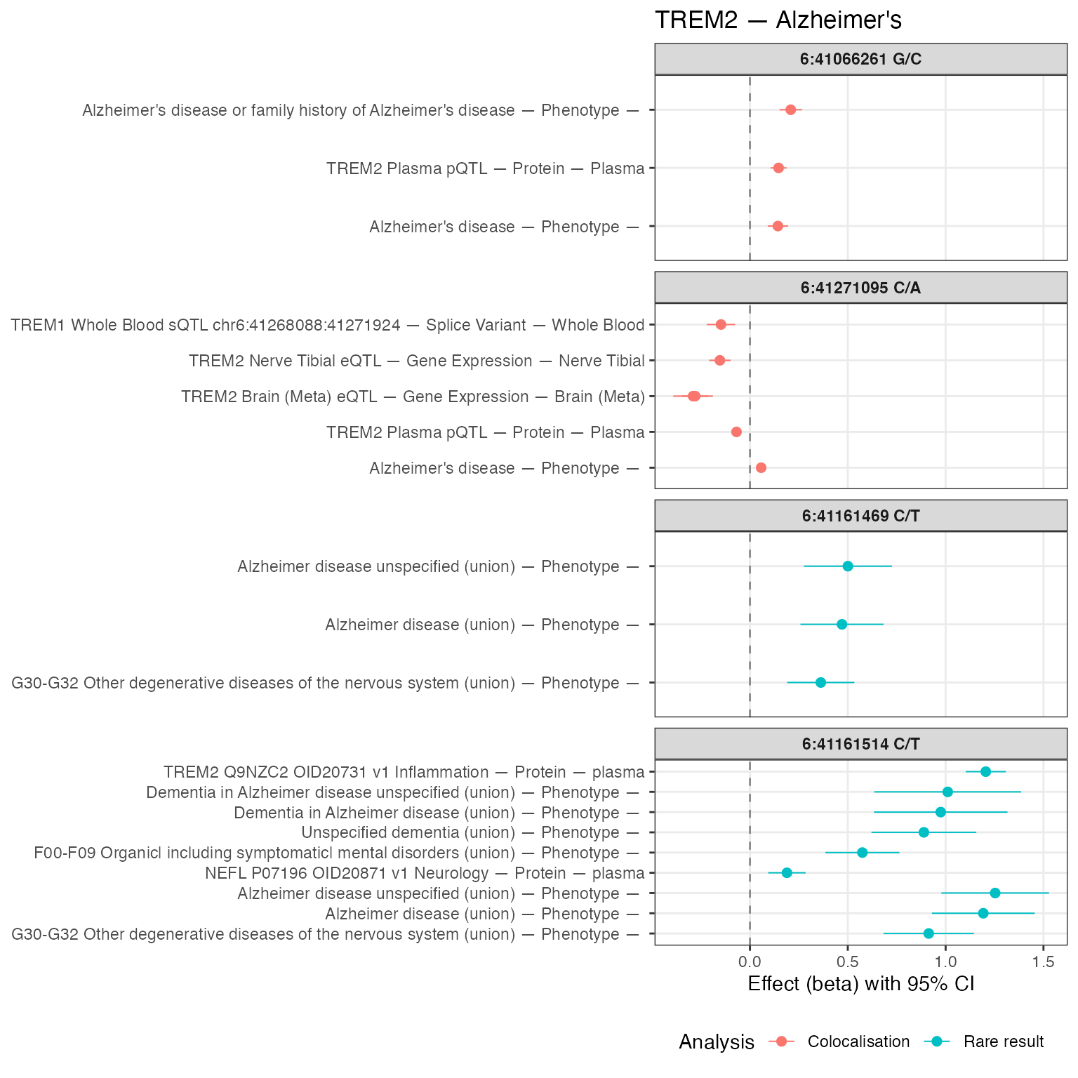

We now have a good overview of the use of TREM2 as a mechanism to investigate, and potentially target for Alzheimer’s disease. We now know:

• TREM2 is associated with Alzheimer’s disease
• TREM2 is associated with two other protein coding genes, TREM1 and TREML2, but there is no evidence of colocalisation with any other nearby genes.
• TREM2 is not associated with any other trait categories, or even any other traits.
• The direction of effect between TREM2 and Alzheimer’s disease seems to be complex. In 3 instances, an increase in the expression of TREM2 is associated with an increase in Alzheimer’s disease, and in 1 instance, a decrease in the expression of TREM2 (across many gene expression, splice variants, and protein levels) is associated with an increase in Alzheimer’s disease.

Existing literature has shown that TREM2 is associated with Alzheimer’s disease, and that TREM2 is currently being investigated as a potential target for Alzheimer’s disease.

Although the GPMap can not provide a definitive answer as a drug target for Alzheimer’s disease, it has proven to helpful in illuminating the potential pleiotropy, and of the directionality of effect that perturbing specific variants associated with TREM2 may have.

Accessing summary statistics

You can only access the summary statistics via variant(), by including include_summary_stats = TRUE in the call. This is to limit the amount of data that can be returned from the API for cost reasons. If you attempt to download too many summary statistics, you may be blocked from the API.

• variant(1669064, include_summary_stats = TRUE)

Instead, if you are interested in accessing all the summary statistics, or the whole database of results, you can download all databases and summary statistics the Google Cloud Storage Bucket, and can find an explanation of the files here. Note that the bucket is ‘requester pays’, so you will need to have a Google Cloud account and be logged in to download the files.