GPMap tutorial: GWAS upload • gpmapr

The GPMap API allows you to upload your own GWAS summary statistics and receive colocalisation results against the existing GPMap. This vignette covers how to upload a GWAS, retrieve your results, interpret them, and compare your upload with another trait (including another upload) to find insights.

Uploading a GWAS

Use gpmapr::upload_gwas() to submit your summary statistics. You need a file with standard GWAS columns and metadata such as sample size and ancestry.

# Example: upload a GWAS file
result <- gpmapr::upload_gwas(
  file = "path/to/your_gwas.tsv.gz",
  name = "Specific Triat",
  p_value_threshold = 5e-8,
  column_names = list(
    CHR = "chr",
    BP = "pos",
    P = "pval",
    EA = "effect_allele",
    OA = "other_allele",
    EAF = "eaf",
    BETA = "beta",
    SE = "se"
  ),
  email = "your@email.com",
  category = "continuous",
  ancestry = "EUR",
  sample_size = 50000,
  reference_build = "GRCh38"
)

You can also compare your upload with another upload by passing the GUIDs of the uploads you want to compare with, by including compare_with_upload_guids = c("GUID1").

The response includes a GUID (a UUID such as a1b2c3d4-e5f6-7890-abcd-ef1234567890). Save this GUID; you use it to fetch your results once they are ready.

# The GUID is returned in the response
my_guid <- result$id

Fetching your results

Processing can take some time. Use the GUID with trait() to check status and retrieve results. Here we will use an GWAS that has already been uploaded to the GPMap.

This is of Atopic Dermatitis.

my_guid <- "7a289615-c1b4-91f3-3d97-887f60de9155"
my_results <- gpmapr::trait(my_guid, include_associations = TRUE)

When processing is complete, the result includes trait, coloc_groups, study_extractions, upload_study_extractions, and optionally associations and coloc_pairs.

Interpreting your results

Much of the same analysis that is shown in the case study can be applied to your upload results. If you are interested in the relationship between your upload and another trait, you can filter the coloc groups by trait id.

Your upload results use the same structure as traits in the database. Here are the main components and what they mean.

Study extractions

The difference between study_extractions and upload_study_extractions is that upload_study_extractions are the individual finemapped regions (LD blocks) that were found from the uploaded GWAS, while study_extractions are the existing finemapped loci that your upload colocalises with.

Key columns include study, snp, gene, chr, bp, min_p, and trait metadata (trait_name, data_type, tissue).

# Study extractions (structure may vary - list of dataframes or single dataframe)
uploaded_study_extractions <- my_results$upload_study_extractions
paste("Number of uploaded study extractions:", nrow(uploaded_study_extractions))
#> [1] "Number of uploaded study extractions: 144"
study_extractions <- my_results$study_extractions
paste("Number of study extractions associated with your upload:", nrow(study_extractions))
#> [1] "Number of study extractions associated with your upload: 3854"

Coloc groups and coloc pairs

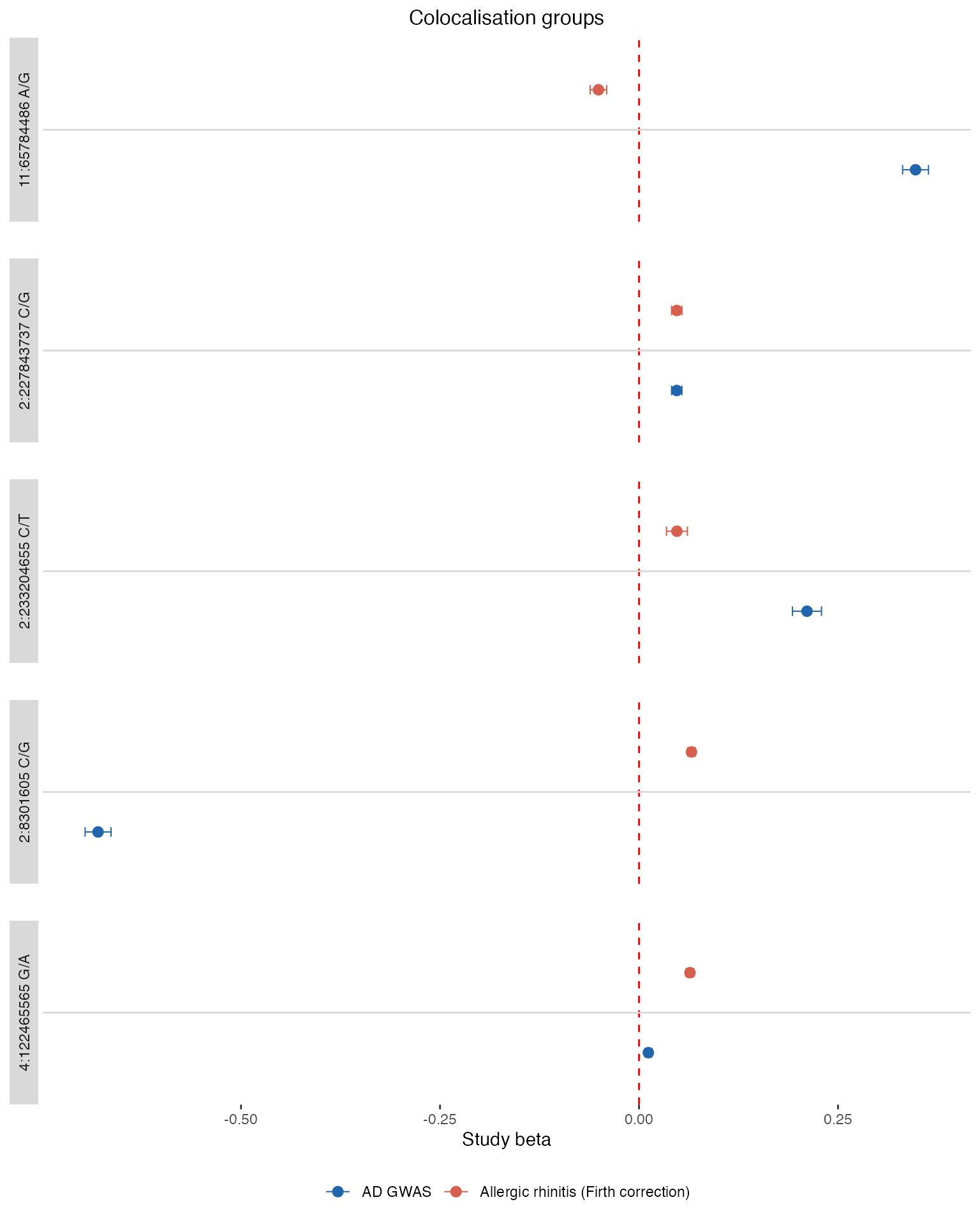
Although coloc groups provide a more robust view of the relationship between your trait and other traits, coloc pairs can be useful for identifying the specific regions that are driving the colocalisation, espeically if the loci is less powered, and therefore less likely to be captured by the coloc groups.

Coloc groups identify genomic regions (LD blocks) where your trait colocalises with other studies in the map. Each row is a study extraction that shares a colocalisation signal with your trait at that region.

If you are interested in the relationship between your trait and another specific trait, you can filter the coloc groups by trait id.

trait_to_compare <- 2527L # Allergic rhinitis
upload_id   <- my_results$trait$id
upload_name <- as.character(my_results$trait$name)[[1L]]

compare_name <- {
  nm <- my_results$coloc_groups |>
    dplyr::filter(trait_id == trait_to_compare) |>
    dplyr::distinct(trait_name) |>
    dplyr::pull(trait_name)
  if (length(nm) >= 1L) nm[[1L]] else "Comparison trait"
}

shared_coloc_groups <- my_results$coloc_groups |>
  dplyr::filter(trait_id == trait_to_compare) |>
  dplyr::pull(coloc_group_id) |>
  unique()

compare_coloc_groups <- my_results$coloc_groups |>
  dplyr::filter(
    coloc_group_id %in% shared_coloc_groups,
    trait_id == trait_to_compare | gwas_upload_id == upload_id
  )

compare_coloc_groups <- compare_coloc_groups |>
  dplyr::group_by(coloc_group_id) |>
  dplyr::filter(!any(se == 1)) |>
  dplyr::ungroup()


# Strongest hit (smallest min_p) per group per side
pick_lead <- function(dat, grp_col) {
  dat |>
    dplyr::filter(!is.na(beta), !is.na(se), se > 0, !is.na(min_p)) |>
    dplyr::group_by(dplyr::across(dplyr::all_of(grp_col))) |>
    dplyr::slice_min(order_by = min_p, n = 1L, with_ties = FALSE) |>
    dplyr::ungroup()
}

trait_colours <- c("#2166ac", "#d6604d")
names(trait_colours) <- c(upload_name, compare_name)

make_forest_plot <- function(df, panel_labels, title_str) {
  lbl_fn <- function(x) {
    m <- match(as.character(x), as.character(panel_labels$group_id))
    out <- panel_labels$strip_lbl[m]
    dplyr::if_else(is.na(out), as.character(x), out)
  }
  ggplot2::ggplot(df, ggplot2::aes(x = beta, y = trait_lbl, colour = trait_lbl)) +
    ggplot2::geom_vline(xintercept = 0, colour = "red", lty = 2) +
    ggplot2::geom_hline(yintercept = 1.5, colour = "grey85", linewidth = 0.5) +
    ggplot2::geom_errorbar(
      ggplot2::aes(xmin = beta - 1.96 * se, xmax = beta + 1.96 * se),
      width = 0.12, linewidth = 0.35
    ) +
    ggplot2::geom_point(size = 2.5) +
    ggplot2::facet_grid(
      rows = ggplot2::vars(coloc_panel),
      scales = "fixed", space = "fixed", switch = "y",
      labeller = ggplot2::labeller(coloc_panel = lbl_fn)
    ) +
    ggplot2::scale_y_discrete(expand = ggplot2::expansion(add = 0.65)) +
    ggplot2::scale_colour_manual(values = trait_colours,
                                 breaks = c(upload_name, compare_name)) +
    ggplot2::theme_bw() +
    ggplot2::theme(
      panel.grid      = ggplot2::element_blank(),
      panel.border    = ggplot2::element_blank(),
      panel.spacing.y = grid::unit(1.5, "lines"),
      strip.background = ggplot2::element_rect(colour = NA),
      strip.placement  = "outside",
      plot.title       = ggplot2::element_text(hjust = 0.5, size = 12),
      legend.position  = "bottom",
      axis.text.y      = ggplot2::element_blank(),
      axis.ticks.y     = ggplot2::element_blank()
    ) +
    ggplot2::labs(x = "Study beta", y = NULL, colour = NULL, title = title_str)
}

make_strip_labels <- function(df) {
  df |>
    dplyr::group_by(group_id) |>
    dplyr::summarise(
      strip_lbl = paste(unique(stats::na.omit(display_snp)), collapse = " · "),
      .groups = "drop"
    ) |>
    dplyr::mutate(strip_lbl = dplyr::if_else(
      nzchar(strip_lbl), strip_lbl, as.character(group_id)
    ))
}

build_forest_df <- function(upload_rows, compare_rows, max_groups = 5L) {
  df <- dplyr::bind_rows(
    upload_rows  |> dplyr::mutate(trait_lbl = upload_name),
    compare_rows |> dplyr::mutate(trait_lbl = compare_name)
  ) |>
    dplyr::mutate(trait_lbl = factor(trait_lbl, levels = c(upload_name, compare_name)))

  ids_both <- df |>
    dplyr::count(group_id, name = "n") |>
    dplyr::filter(n == 2L) |>
    dplyr::slice_head(n = max_groups) |>
    dplyr::pull(group_id)

  df |>
    dplyr::filter(group_id %in% ids_both) |>
    dplyr::mutate(coloc_panel = factor(group_id))
}

# --- Section 1: Coloc groups ---
cg_upload <- compare_coloc_groups |>
  dplyr::filter(gwas_upload_id == upload_id) |>
  pick_lead("coloc_group_id") |>
  dplyr::mutate(group_id = as.character(coloc_group_id))

cg_compare <- compare_coloc_groups |>
  dplyr::filter(trait_id == trait_to_compare) |>
  pick_lead("coloc_group_id") |>
  dplyr::mutate(group_id = as.character(coloc_group_id))

cg_df <- build_forest_df(cg_upload, cg_compare)

if (nrow(cg_df) > 0) {
  print(make_forest_plot(
    cg_df, make_strip_labels(cg_df),
    "Colocalisation groups"
  ))
}


# --- Section 2: Coloc pairs only (h4 > 0.8, locus not in shared coloc groups) ---
pairs_all <- my_results$coloc_pairs

if (!is.null(pairs_all) && nrow(pairs_all) > 0 && "h4" %in% names(pairs_all) &&
    "ld_block_id" %in% names(pairs_all)) {
  covered_ld <- compare_coloc_groups |>
    dplyr::pull(ld_block_id) |>
    unique()

  sig_ld <- pairs_all |>
    dplyr::filter(h4 > 0.8, !ld_block_id %in% covered_ld) |>
    dplyr::pull(ld_block_id) |>
    unique()

  if (length(sig_ld) > 0) {
    cp_upload <- my_results$coloc_groups |>
      dplyr::filter(gwas_upload_id == upload_id, ld_block_id %in% sig_ld) |>
      pick_lead("ld_block_id") |>
      dplyr::mutate(group_id = as.character(ld_block_id))

    cp_compare <- my_results$coloc_groups |>
      dplyr::filter(trait_id == trait_to_compare, ld_block_id %in% sig_ld) |>
      pick_lead("ld_block_id") |>
      dplyr::mutate(group_id = as.character(ld_block_id))

    cp_df <- build_forest_df(cp_upload, cp_compare)

    if (nrow(cp_df) > 0) {
      print(make_forest_plot(
        cp_df, make_strip_labels(cp_df),
        "Coloc pairs only (h4 > 0.8, not in a shared coloc group)"
      ))
    }
  }
}

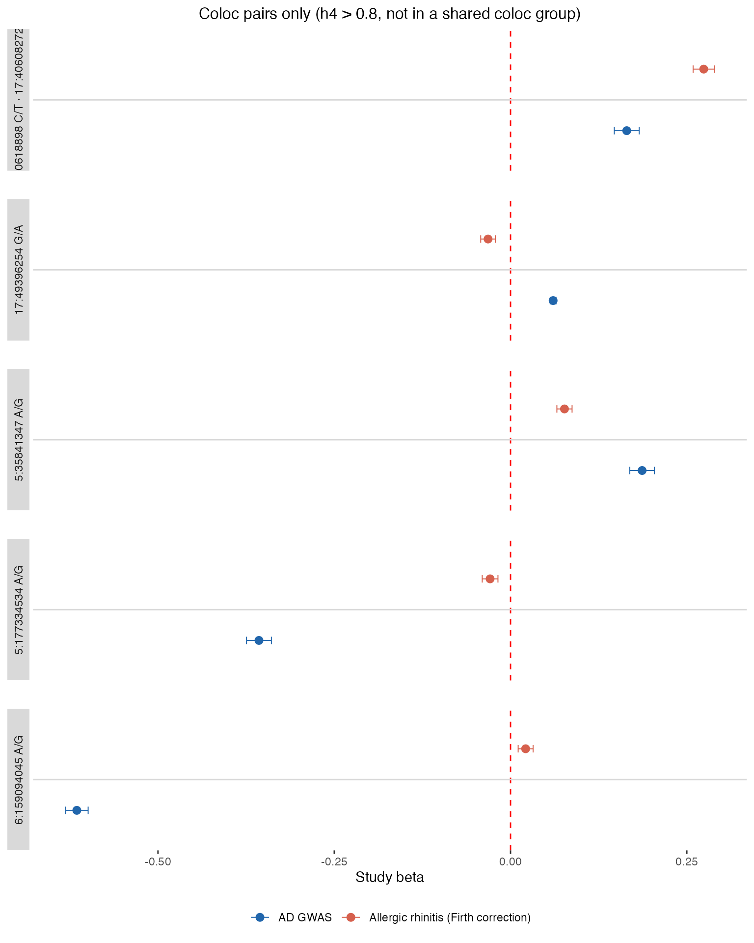
Coloc pairs give pairwise colocalisation probabilities between study extractions:

h4: Both traits share one common causal variant
h3: Both traits associate at the region through two distinct causal variants

The forest plot above already includes loci with h4 > 0.8 that are not captured by any shared coloc group. The raw pair scores for all significant pairs are shown below.

truncate_results <- 20L

pairs <- my_results$coloc_pairs
if (!is.null(pairs) && nrow(pairs) > 0) {
  cols <- intersect(names(pairs), c(
    "study_extraction_id_a", "study_extraction_id_b",
    "existing_study_extraction_id_a", "existing_study_extraction_id_b",
    "ld_block_id", "h3", "h4", "false_positive", "spurious"
  ))
  knitr::kable(
    head(dplyr::filter(pairs[, cols, drop = FALSE], h4 > 0.8), truncate_results),
    digits = 3
  )
} else {
  "No coloc pairs for these traits"
}

existing_study_extraction_id_a	study_extraction_id_a	existing_study_extraction_id_b	study_extraction_id_b	ld_block_id	h3	h4	false_positive
NA	7293	46415	NA	9	0.083	0.882	FALSE
NA	7293	49939	NA	9	0.117	0.879	FALSE
NA	7293	50071	NA	9	0.003	0.996	FALSE
NA	7293	50085	NA	9	0.086	0.911	FALSE
NA	7294	276438	NA	58	0.002	0.998	FALSE
NA	7294	276555	NA	58	0.069	0.931	FALSE
NA	7294	276582	NA	58	0.002	0.998	FALSE
NA	7295	NA	7296	59	0.000	1.000	FALSE
NA	7297	NA	7298	59	0.000	1.000	FALSE
NA	7303	281882	NA	60	0.067	0.933	FALSE
NA	7303	282948	NA	60	0.064	0.936	FALSE
NA	7303	283008	NA	60	0.071	0.929	FALSE
NA	7303	283259	NA	60	0.057	0.943	FALSE
NA	7303	289880	NA	60	0.097	0.903	FALSE
NA	7303	291699	NA	60	0.047	0.952	FALSE
NA	7303	291703	NA	60	0.127	0.872	FALSE
NA	7303	296454	NA	60	0.039	0.960	FALSE
NA	7303	296463	NA	60	0.052	0.948	FALSE
NA	7303	296756	NA	60	0.025	0.975	FALSE
NA	7303	296758	NA	60	0.047	0.953	FALSE