Genetic colocalisation • gwasglue

Here we’ll perform colocalisation analysis for a particular region, and plot the regions as well. We’ll do the same analysis two ways:

querying the association data from the IEU GWAS database, and
downloading the GWAS VCF files and querying those.

We’ll use the example of LDL cholesterol ieu-a-300 and coronary heart disease ieu-a-7.

Load libraries:

suppressPackageStartupMessages(suppressWarnings({
    library(gwasglue)
    library(dplyr)
    library(gassocplot)
    library(coloc)
}))
#> API: public: http://gwas-api.mrcieu.ac.uk/

ieugwasr

First find a region that we know to be associated with LDL cholesterol.

top <- ieugwasr::tophits('ieu-a-300') %>% arrange(p)
top
#> # A tibble: 81 x 12
#>       beta position     se         p chr        n id    rsid  ea    nea      eaf
#>      <dbl>    <int>  <dbl>     <dbl> <chr>  <int> <chr> <chr> <chr> <chr>  <dbl>
#>  1 -0.150    1.10e8 0.0047 1.00e-200 1     172825 ieu-… rs49… T     C     0.187 
#>  2 -0.221    1.12e7 0.0061 1.00e-200 19    170608 ieu-… rs65… T     G     0.0976
#>  3 -0.485    4.54e7 0.0119 1.00e-200 19    139198 ieu-… rs72… A     G     0.0317
#>  4  0.119    2.13e7 0.004  9.48e-183 2     173007 ieu-… rs13… A     G     0.288 
#>  5 -0.497    5.55e7 0.018  8.57e-143 1      77417 ieu-… rs11… T     G     0.0172
#>  6 -0.446    4.54e7 0.0183 2.99e-122 19     99409 ieu-… rs12… A     G     0.0172
#>  7 -0.0806   4.41e7 0.0041 4.84e- 83 2     172940 ieu-… rs65… C     T     0.706 
#>  8  0.0733   7.47e7 0.0038 7.79e- 78 5     168357 ieu-… rs12… C     T     0.431 
#>  9 -0.189    4.52e7 0.0112 7.29e- 62 19    170260 ieu-… rs29… C     T     0.0211
#> 10 -0.0564   1.26e8 0.0036 2.10e- 50 8     172963 ieu-… rs29… T     A     0.468 
#> # … with 71 more rows, and 1 more variable: trait <chr>

Choose the best signal and create a range

chrpos <- paste0(top$chr[1], ":", top$position[1] - 90000, "-", top$position[1] + 90000)
chrpos
#> [1] "1:109724880-109904880"

Extract, harmonise and format the data

out <- ieugwasr_to_coloc(id1='ieu-a-300', id2='ieu-a-7', chrompos=chrpos)

Run colocalisation analysis

res <- coloc::coloc.abf(out[[1]], out[[2]])
#> Warning in sdY.est(d$varbeta, d$MAF, d$N): estimating sdY from maf and varbeta,
#> please directly supply sdY if known
#> PP.H0.abf PP.H1.abf PP.H2.abf PP.H3.abf PP.H4.abf 
#> 1.31e-304  1.29e-19 3.67e-288  2.61e-03  9.97e-01 
#> [1] "PP abf for shared variant: 99.7%"

Plot

temp <- coloc_to_gassocplot(out)
#> Extracting LD matrix for 253 variants
#> Please look at vignettes for options on running this locally if you need to run many instances of this command.
#> Warning in ieugwasr::ld_matrix(markers[["marker"]], with_alleles = FALSE, : The following variants are not present in the LD reference panel
#> rs114570757
#> rs115867281
#> rs116711509
#> rs3850615
#> rs41279710
#> rs41279722
#> rs6683212
#> Found 246 variants in LD reference panel
gassocplot::stack_assoc_plot(temp$markers, temp$z, temp$corr, traits=temp$traits)

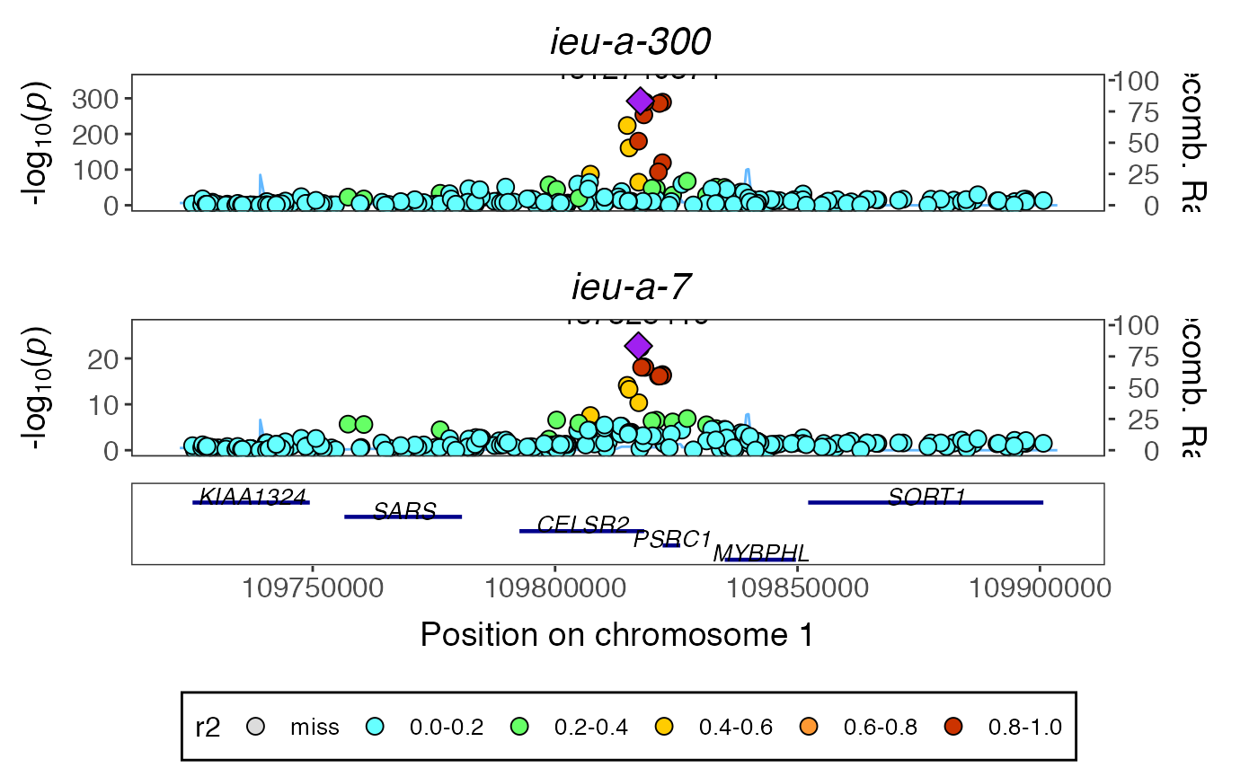
#> TableGrob (2 x 1) "arrange": 2 grobs
#>   z     cells    name              grob
#> 1 1 (1-1,1-1) arrange    gtable[layout]
#> 2 2 (2-2,1-1) arrange gtable[guide-box]

gwasvcf

Let’s do the same with the vcf files (and the indexes). Download from here:

Set a region to plot:

chrpos <- "19:11112306-11292306"

Extract region from vcf files and convert to coloc object

vout <- gwasvcf_to_coloc("ieu-a-300.vcf.gz", "ieu-a-7.vcf.gz", chrpos)
#> 'tools_bcftools' option is not set, using native read which may be substantially slower. See 'set_bcftools' for information.
#> 'tools_bcftools' option is not set, using native read which may be substantially slower. See 'set_bcftools' for information.

Run colocalisation analysis

vres <- coloc::coloc.abf(vout[[1]], vout[[2]])
#> Warning in sdY.est(d$varbeta, d$MAF, d$N): estimating sdY from maf and varbeta,
#> please directly supply sdY if known

#> Warning in sdY.est(d$varbeta, d$MAF, d$N): estimating sdY from maf and varbeta,
#> please directly supply sdY if known
#> PP.H0.abf PP.H1.abf PP.H2.abf PP.H3.abf PP.H4.abf 
#> 3.85e-289  3.38e-10 7.35e-281  6.35e-02  9.36e-01 
#> [1] "PP abf for shared variant: 93.6%"

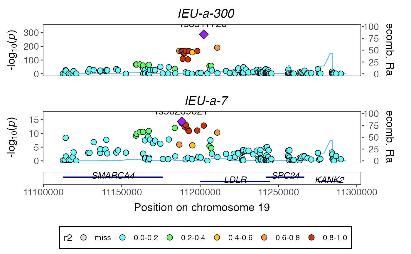
Plot

library(gassocplot)
temp <- coloc_to_gassocplot(vout)
#> Extracting LD matrix for 148 variants
#> Please look at vignettes for options on running this locally if you need to run many instances of this command.
#> Warning in ieugwasr::ld_matrix(markers[["marker"]], with_alleles = FALSE, : The following variants are not present in the LD reference panel
#> rs8110695
#> rs2738459
#> rs17001200
#> Found 145 variants in LD reference panel
gassocplot::stack_assoc_plot(temp$markers, temp$z, temp$corr, traits=temp$traits)

#> TableGrob (2 x 1) "arrange": 2 grobs
#>   z     cells    name              grob
#> 1 1 (1-1,1-1) arrange    gtable[layout]
#> 2 2 (2-2,1-1) arrange gtable[guide-box]