Tutorial • CAMeRa

library(CAMeRa)

Introduction

This software attempts to bring together various tools to improve cross-ancestry Mendelian randomisation. It will use an example of performing analysis of BMI on coronary heart disease across four major ancestral groups.

Overview:

Initialise data
Check phenotype scales across ancestries
Extract instruments
Evaluate instrument heterogeneity across populations
Extract outcome data
Harmonise exposure and outcome data
Perform analysis using raw instruments
Perform regional scan to obtain LD agnostic instruments
Re-perform analysis using regional instruments
Evaluate similarity of pleiotropy across ancestry
Evaluate similarity of instrument-exposure associations
Use cross-population instrument-exposure heterogeneity in MR GxE framework to estimate pleiotropy distributions
Saving and loading data

Initialise data

CAMeRa begins by choosing an exposure and outcome hypothesis that can be tested in multi-ancestral populations. Here, we will be estimating the causal effect of body mass index (BMI) on coronary heart disease (CHD) in European (EUR), East Asian (EAS), African (AFR) and South Asian (SAS) ancestries.

Summary statistics data can be extracted from the IEU GWAS database using the TwoSampleMR package. A list of available traits can be obtained using:

traits <- TwoSampleMR::available_outcomes()

You can also browse the available traits here: https://gwas.mrcieu.ac.uk/. Also see other vignettes on this site about how you can use local summary statistics instead.

Querying the OpenGWAS API requires an access token, see the ieugwasr guide for how to obtain and set one up. The examples in this vignette make many API queries and so may use up a large part of your allowance. To keep this vignette fast to build, the code chunks that query the API are not run here, instead the results are loaded from an example object that ships with the package.

Once you obtain the study IDs for the exposure and the outcome, open R6 class environment to run CAMERA. The minimum information required for CAMERA is the following:

Summary statistics for the exposure and the outcome
Population information
Plink (version 1.90)
LD reference data

Plink (version 1.90) and LD reference data are required to identify instruments that can be used for both populations. LD reference data can be accessed from: http://fileserve.mrcieu.ac.uk/ld/1kg.v3.tgz.

The example below uses the genetics.binaRies package to locate a plink executable. It is not installed with CAMeRa, so either install it with

install.packages("genetics.binaRies", repos = c("https://mrcieu.r-universe.dev", "https://cloud.r-project.org"))

or set plink to the path of your own plink executable.

bfile_dir <- "/path/to/ld_files"
x <- CAMERA$new(
  exposure_ids=c(
    "ukb-e-23104_CSA", 
    "ukb-e-21001_AFR", 
    "ukb-b-19953", 
    "bbj-a-1"
  ), 
  outcome_ids=c(
    "ukb-e-411_CSA", 
    "ukb-e-411_AFR", 
    "ieu-a-7", 
    "bbj-a-109"
  ), 
  pops = c("SAS", "AFR", "EUR", "EAS"),
  bfiles=file.path(bfile_dir, c("SAS", "AFR", "EUR", "EAS")),
  plink = genetics.binaRies::get_plink_binary(),        
  radius=50000, 
  clump_pop="EUR"
)
x

In this vignette the code chunks that query OpenGWAS or need plink are shown but not run. Instead, we load the results of running them from an example object that ships with the package. This object was created in September 2026. The data in OpenGWAS can change over time, so if you run the analysis yourself your results may differ from those shown here.

x_example <- readRDS(system.file(package="CAMeRa", "extdata/example-CAMERA.rds"))
x <- CAMERA$new()
x$import(x_example)
rm(x_example)

Check phenotype scales across ancestries

Make sure that the exposures/outcomes are matched across the populations. The different populations should have the same exposure-outcome pair, with exposure and outcome traits measured in the same way and with the same units. Also, instrument-trait associations should be consistent between the populations (e.g. how similar SNP-BMI association in EUR to SNP-BMI association in EAS). You can check this as follows:

x$check_phenotypes(ids=x$exposure_ids)
x$check_phenotypes(ids=x$outcome_ids)

Extract instruments

We can now perform the analysis, which will do the following:

Extract instruments for the exposures
Check the validity of the instruments across the populations (Standardise/scale the data if necessary)
Extract new instruments based on LD information and fine-mapping
Extract instruments for the outcomes
Harmonise the exposure data and the outcome data
Perform MR

See ?CAMERA, or the CAMERA reference page, for details of the options and outputs of each method. A summary of the methods used in this vignette is given in the Overview of methods section at the end.

The following function identifies SNPs that have strong associations with the exposure in each population. This is the same method as instrument extraction for multivariable MR.

x$extract_instruments()

A data frame of the extracted instruments is stored in x$instrument_raw

str(x$instrument_raw)
#> 'data.frame':    1528 obs. of  14 variables:
#>  $ rsid      : chr  "1:2723214_A_C" "1:6657424_A_C" "1:11207269_C_T" "1:19934900_A_G" ...
#>  $ chr       : chr  "1" "1" "1" "1" ...
#>  $ position  : int  2723214 6657424 11207269 19934900 23313353 33784146 39564930 47678458 49996959 66434743 ...
#>  $ id        : chr  "ukb-e-23104_CSA" "ukb-e-23104_CSA" "ukb-e-23104_CSA" "ukb-e-23104_CSA" ...
#>  $ beta      : num  -0.0266 -0.0235 0.0171 -0.0148 -0.0169 ...
#>  $ se        : num  0.0154 0.0154 0.0192 0.0169 0.0146 ...
#>  $ p         : num  0.0841 0.1262 0.3728 0.3823 0.2496 ...
#>  $ ea        : chr  "A" "A" "C" "A" ...
#>  $ nea       : chr  "C" "C" "T" "G" ...
#>  $ eaf       : num  0.33 0.324 0.166 0.234 0.578 ...
#>  $ units     : chr  "NA" "NA" "NA" "NA" ...
#>  $ samplesize: num  8658 8658 8658 8658 8658 ...
#>  $ method    : chr  "raw" "raw" "raw" "raw" ...
#>  $ rsido     : chr  "rs4648450" "rs3866805" "rs2791643" "rs61740466" ...

Evaluate instrument heterogeneity across populations

It is important to ensure that the instruments for the exposure are valid across the populations. Once instruments for the exposure trait are identified for each population, we can assess specificity of the instruments. Each of the following functions estimates heterogeneity of the instruments between and calculates fraction of the instruments (obtained from the Step 1) that are replicated between the populations.

x$instrument_heterogeneity()
#> # A tibble: 6 × 9
#>   Reference Replication  nsnp agreement     se      pval     I2      Q    Q_pval
#>   <chr>     <chr>       <int>     <dbl>  <dbl>     <dbl>  <dbl>  <dbl>     <dbl>
#> 1 ukb-b-19… ukb-e-2310…   373     0.676 0.0478 2.78e- 45 0.0315  385.  3.09e-  1
#> 2 ukb-b-19… ukb-e-2100…   373     0.476 0.0683 3.35e- 12 0.103   416.  5.85e-  2
#> 3 ukb-b-19… bbj-a-1       373     0.578 0.0210 3.97e-166 0.635  1022.  5.75e- 62
#> 4 bbj-a-1   ukb-e-2310…    46     0.761 0.0932 3.15e- 16 0.176    55.8 1.29e-  1
#> 5 bbj-a-1   ukb-e-2100…    46     0.518 0.144  3.31e-  4 0.354    71.2 7.69e-  3
#> 6 bbj-a-1   ukb-b-19953    46     0.843 0.0544 5.12e- 54 0.953   975.  5.68e-175

x$estimate_instrument_specificity(instrument=x$instrument_raw)
#> Checking ukb-e-23104_CSA against ukb-e-21001_AFR
#> Checking ukb-e-23104_CSA against ukb-b-19953
#> Checking ukb-e-23104_CSA against bbj-a-1
#> Checking ukb-e-21001_AFR against ukb-e-23104_CSA
#> Checking ukb-e-21001_AFR against ukb-b-19953
#> Checking ukb-e-21001_AFR against bbj-a-1
#> Checking ukb-b-19953 against ukb-e-23104_CSA
#> Checking ukb-b-19953 against ukb-e-21001_AFR
#> Checking ukb-b-19953 against bbj-a-1
#> Checking bbj-a-1 against ukb-e-23104_CSA
#> Checking bbj-a-1 against ukb-e-21001_AFR
#> Checking bbj-a-1 against ukb-b-19953
#>          discovery     replication nsnp  metric    datum       value
#> 1  ukb-e-21001_AFR ukb-e-23104_CSA    1 P-value Expected   0.9987758
#> 2  ukb-e-21001_AFR ukb-e-23104_CSA    1 P-value Observed   1.0000000
#> 3  ukb-e-21001_AFR ukb-e-23104_CSA    1    Sign Expected   0.9999995
#> 4  ukb-e-21001_AFR ukb-e-23104_CSA    1    Sign Observed   1.0000000
#> 5  ukb-e-21001_AFR     ukb-b-19953    1 P-value Expected   1.0000000
#> 6  ukb-e-21001_AFR     ukb-b-19953    1 P-value Observed   1.0000000
#> 7  ukb-e-21001_AFR     ukb-b-19953    1    Sign Expected   0.9999995
#> 8  ukb-e-21001_AFR     ukb-b-19953    1    Sign Observed   1.0000000
#> 9  ukb-e-21001_AFR         bbj-a-1    1 P-value Expected   1.0000000
#> 10 ukb-e-21001_AFR         bbj-a-1    1 P-value Observed   1.0000000
#> 11 ukb-e-21001_AFR         bbj-a-1    1    Sign Expected   0.9999995
#> 12 ukb-e-21001_AFR         bbj-a-1    1    Sign Observed   1.0000000
#> 13     ukb-b-19953 ukb-e-23104_CSA  373 P-value Expected   1.7599653
#> 14     ukb-b-19953 ukb-e-23104_CSA  373 P-value Observed   2.0000000
#> 15     ukb-b-19953 ukb-e-23104_CSA  373    Sign Expected 311.1377768
#> 16     ukb-b-19953 ukb-e-23104_CSA  373    Sign Observed 270.0000000
#> 17     ukb-b-19953 ukb-e-21001_AFR  373 P-value Expected   0.4125545
#> 18     ukb-b-19953 ukb-e-21001_AFR  373 P-value Observed   1.0000000
#> 19     ukb-b-19953 ukb-e-21001_AFR  373    Sign Expected 281.1770175
#> 20     ukb-b-19953 ukb-e-21001_AFR  373    Sign Observed 232.0000000
#> 21     ukb-b-19953         bbj-a-1  373 P-value Expected 127.0276153
#> 22     ukb-b-19953         bbj-a-1  373 P-value Observed  41.0000000
#> 23     ukb-b-19953         bbj-a-1  373    Sign Expected 368.2446361
#> 24     ukb-b-19953         bbj-a-1  373    Sign Observed 327.0000000
#> 25         bbj-a-1 ukb-e-23104_CSA   46 P-value Expected   1.4318562
#> 26         bbj-a-1 ukb-e-23104_CSA   46 P-value Observed   2.0000000
#> 27         bbj-a-1 ukb-e-23104_CSA   46    Sign Expected  42.1873456
#> 28         bbj-a-1 ukb-e-23104_CSA   46    Sign Observed  40.0000000
#> 29         bbj-a-1 ukb-e-21001_AFR   46 P-value Expected   0.2499113
#> 30         bbj-a-1 ukb-e-21001_AFR   46 P-value Observed   1.0000000
#> 31         bbj-a-1 ukb-e-21001_AFR   46    Sign Expected  38.9215168
#> 32         bbj-a-1 ukb-e-21001_AFR   46    Sign Observed  29.0000000
#> 33         bbj-a-1     ukb-b-19953   46 P-value Expected  45.3411632
#> 34         bbj-a-1     ukb-b-19953   46 P-value Observed  38.0000000
#> 35         bbj-a-1     ukb-b-19953   46    Sign Expected  45.9998778
#> 36         bbj-a-1     ukb-b-19953   46    Sign Observed  45.0000000
#>           pdiff
#> 1  1.000000e+00
#> 2  1.000000e+00
#> 3  1.000000e+00
#> 4  1.000000e+00
#> 5  1.000000e+00
#> 6  1.000000e+00
#> 7  1.000000e+00
#> 8  1.000000e+00
#> 9  1.000000e+00
#> 10 1.000000e+00
#> 11 1.000000e+00
#> 12 1.000000e+00
#> 13 6.970256e-01
#> 14 6.970256e-01
#> 15 9.115926e-08
#> 16 9.115926e-08
#> 17 3.381940e-01
#> 18 3.381940e-01
#> 19 1.735794e-08
#> 20 1.735794e-08
#> 21 1.063832e-24
#> 22 1.063832e-24
#> 23 2.350641e-30
#> 24 2.350641e-30
#> 25 6.549345e-01
#> 26 6.549345e-01
#> 27 2.748258e-01
#> 28 2.748258e-01
#> 29 2.216606e-01
#> 30 2.216606e-01
#> 31 2.921155e-04
#> 32 2.921155e-04
#> 33 2.843716e-07
#> 34 2.843716e-07
#> 35 1.221987e-04
#> 36 1.221987e-04

Extract outcome data

x$make_outcome_data()

Harmonise exposure and outcome data

x$harmonise()
#> # A tibble: 4 × 4
#>   pops  exposure_ids    outcome_ids   source  
#>   <chr> <chr>           <chr>         <chr>   
#> 1 SAS   ukb-e-23104_CSA ukb-e-411_CSA OpenGWAS
#> 2 AFR   ukb-e-21001_AFR ukb-e-411_AFR OpenGWAS
#> 3 EUR   ukb-b-19953     ieu-a-7       OpenGWAS
#> 4 EAS   bbj-a-1         bbj-a-109     OpenGWAS
#> 'data.frame':    1528 obs. of  4 variables:
#>  $ SNP : chr  "1:2723214_A_C" "1:6657424_A_C" "1:11207269_C_T" "1:19934900_A_G" ...
#>  $ pops: chr  "SAS" "SAS" "SAS" "SAS" ...
#>  $ beta: num  -0.0266 -0.0235 0.0171 -0.0148 -0.0169 ...
#>  $ se  : num  0.0154 0.0154 0.0192 0.0169 0.0146 ...
#> NULL
#> 'data.frame':    2911 obs. of  4 variables:
#>  $ SNP : chr  "1:11207269_C_T" "1:11207269_C_T" "1:11207269_C_T" "1:11207269_C_T" ...
#>  $ pops: chr  "EAS" "EUR" "AFR" "SAS" ...
#>  $ beta: num  0.023401 -0.003275 -0.09457 -0.06663 0.000183 ...
#>  $ se  : num  0.0319 0.0112 0.0809 0.0594 0.016 ...
#> NULL
#> 'data.frame':    1507 obs. of  6 variables:
#>  $ SNP   : chr  "1:2723214_A_C" "1:6657424_A_C" "1:11207269_C_T" "1:19934900_A_G" ...
#>  $ pops  : chr  "SAS" "SAS" "SAS" "SAS" ...
#>  $ beta.x: num  -0.0266 -0.0235 0.0171 -0.0148 -0.0169 ...
#>  $ se.x  : num  0.0154 0.0154 0.0192 0.0169 0.0146 ...
#>  $ beta.y: num  -0.0152 -0.0295 -0.0666 0.0603 0.0465 ...
#>  $ se.y  : num  0.048 0.0479 0.0594 0.0527 0.0456 ...
#> NULL

Perform analysis using raw instruments

We will perform an inverse variance weighted fixed effects MR method within population and across all populations. Heterogeneity estimates will be generated to evaluate if each population has a distinct association compared to others. The combined estimate across all populations assumes that the effect is drawn from the same distribution and if that assumption holds then then power is improved because of the combined information.

x$cross_estimate()
#> # A tibble: 5 × 8
#>   pops  Estimate `Std. Error` `t value` `Pr(>|t|)`    Qj Qjpval   Qdf
#>   <chr>    <dbl>        <dbl>     <dbl>      <dbl> <dbl>  <dbl> <dbl>
#> 1 All      0.443       0.0292    15.2     1.27e-48 8.02  0.0456     3
#> 2 AFR      0.131       0.214      0.613   5.40e- 1 2.12  0.145      1
#> 3 EAS      0.611       0.0745     8.20    4.97e-16 5.09  0.0241     1
#> 4 EUR      0.423       0.0329    12.9     5.81e-36 0.374 0.541      1
#> 5 SAS      0.353       0.136      2.59    9.57e- 3 0.441 0.506      1

In this example the estimates are broadly similar across ancestries, although the EAS estimate is somewhat larger than the others and the AFR estimate is smaller and imprecise (see the Qjpval column), and the Qjpval of the All row gives some evidence of heterogeneity across the populations. Note that the All estimate is more precisely estimated than any of the others because it is combining the information across populations.

We can visualise the estimates:

x$plot_cross_estimate()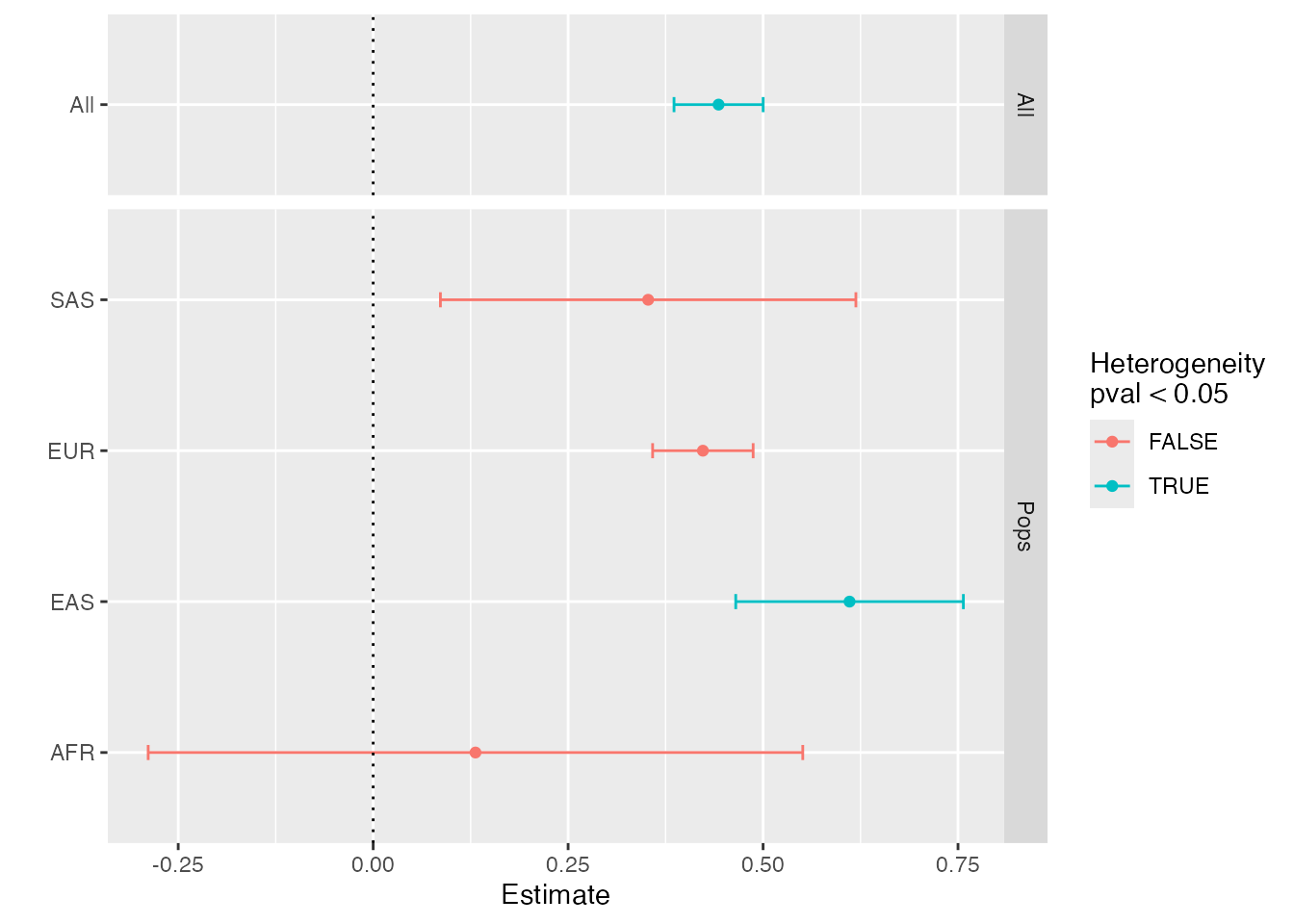

Perform regional scan to obtain LD agnostic instruments

We can re-select the instruments scanning across the region. The intention here is to allow all populations to contribute to a fixed effects meta analysis to account for LD. Then the top variant in the region from the meta analysis is used as the instrument for all populations.

x$extract_instrument_regions()

This has extracted regions around all the pooled instruments from each exposure dataset. Now we can choose the best SNP in each region across all ancestries using a fixed effects meta analysis. For the cases where the most strongly associated SNPs are not available at exactly the same position, the function searches alternative SNPs that are located near the original SNP and show the largest effect size magnitude.

x$fema_regional_instruments() %>% str()
#> tibble [1,524 × 13] (S3: tbl_df/tbl/data.frame)
#>  $ id      : chr [1:1524] "ukb-e-23104_CSA" "ukb-e-21001_AFR" "ukb-b-19953" "bbj-a-1" ...
#>  $ trait   : chr [1:1524] "Body mass index (BMI)" "Body mass index (BMI)" "Body mass index (BMI)" "Body mass index" ...
#>  $ chr     : chr [1:1524] "1" "1" "1" "1" ...
#>  $ position: int [1:1524] 2722848 2722848 2722848 2722848 6694927 6694927 6694927 6694927 11236410 11236410 ...
#>  $ rsid    : chr [1:1524] "1:2722848_C_T" "1:2722848_C_T" "1:2722848_C_T" "1:2722848_C_T" ...
#>  $ ea      : chr [1:1524] "C" "C" "C" "C" ...
#>  $ nea     : chr [1:1524] "T" "T" "T" "T" ...
#>  $ eaf     : num [1:1524] 0.715 0.859 0.534 0.565 0.714 ...
#>  $ beta    : num [1:1524] 0.0174 -0.0312 0.0144 0.012 0.0258 ...
#>  $ se      : num [1:1524] 0.01609 0.02562 0.00199 0.00422 0.01579 ...
#>  $ p       : num [1:1524] 2.80e-01 2.24e-01 5.10e-13 4.33e-03 1.02e-01 ...
#>  $ n       : num [1:1524] NA NA 461460 NA NA ...
#>  $ rsido   : chr [1:1524] "rs6692145" "rs6692145" "rs6692145" "rs6692145" ...

Alternatively, use a Z-score based meta analysis if you are unsure about whether the effect size scales are sufficiently consistent across the studies:

x$fema_regional_instruments(method="zma") %>% str()
#> tibble [1,524 × 13] (S3: tbl_df/tbl/data.frame)
#>  $ id      : chr [1:1524] "ukb-e-23104_CSA" "ukb-e-21001_AFR" "ukb-b-19953" "bbj-a-1" ...
#>  $ trait   : chr [1:1524] "Body mass index (BMI)" "Body mass index (BMI)" "Body mass index (BMI)" "Body mass index" ...
#>  $ chr     : chr [1:1524] "1" "1" "1" "1" ...
#>  $ position: int [1:1524] 2722848 2722848 2722848 2722848 6684906 6684906 6684906 6684906 11236410 11236410 ...
#>  $ rsid    : chr [1:1524] "1:2722848_C_T" "1:2722848_C_T" "1:2722848_C_T" "1:2722848_C_T" ...
#>  $ ea      : chr [1:1524] "C" "C" "C" "C" ...
#>  $ nea     : chr [1:1524] "T" "T" "T" "T" ...
#>  $ eaf     : num [1:1524] 0.715 0.859 0.534 0.565 0.702 ...
#>  $ beta    : num [1:1524] 0.0174 -0.0312 0.0144 0.012 0.027 ...
#>  $ se      : num [1:1524] 0.01609 0.02562 0.00199 0.00422 0.01562 ...
#>  $ p       : num [1:1524] 2.80e-01 2.24e-01 5.10e-13 4.33e-03 8.35e-02 ...
#>  $ n       : num [1:1524] NA NA 461460 NA NA ...
#>  $ rsido   : chr [1:1524] "rs6692145" "rs6692145" "rs6692145" "rs6692145" ...

Example

x$plot_regional_instruments(names(x$instrument_regions)[3])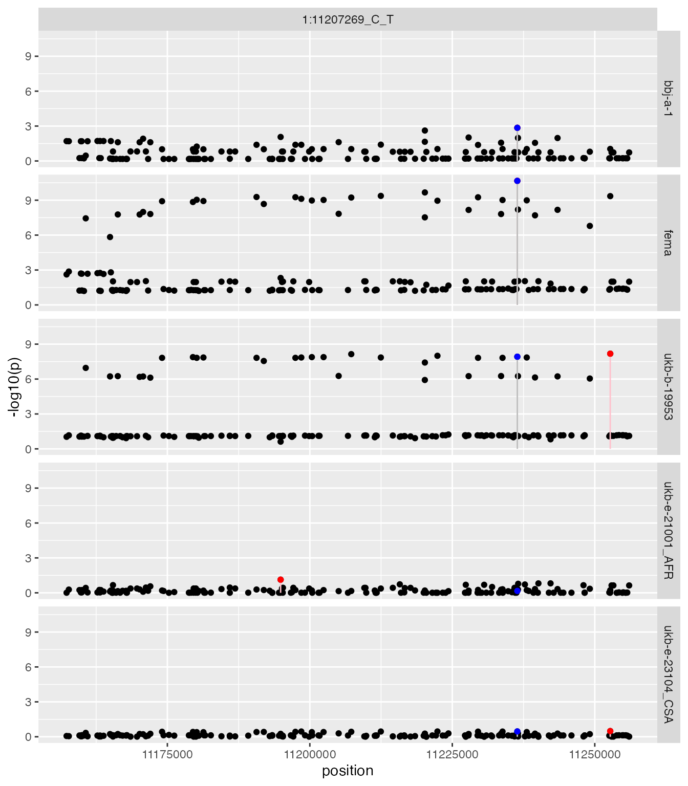

Here, the European top hit is in LD with many other variants in the European ancestry, but meta-analysing with the other ancestries identified a similarly strongly associated variant in Europeans that is also strongly associated in East Asians. Had we used the European top hit then we would have missed the stronger association in the region that associates with other ancestries too. Note that the sample sizes for the SAS and AFR studies are very small and relatively underpowered throughout the analysis.

Re-perform analysis using regional instruments

We now repeat the analysis using the regional instruments in x$instrument_fema. First, extract outcome data for the regional instruments. Outcome data are only extracted for SNPs which are not already in x$instrument_outcome, and are appended to it, so the existing outcome data are kept.

x$make_outcome_data(exp=x$instrument_fema)

Re-harmonise using the regional instruments. This replaces x$harmonised_dat, so the analyses below use the regional instruments.

x$harmonise(exp=x$instrument_fema)
#> # A tibble: 4 × 4
#>   pops  exposure_ids    outcome_ids   source  
#>   <chr> <chr>           <chr>         <chr>   
#> 1 SAS   ukb-e-23104_CSA ukb-e-411_CSA OpenGWAS
#> 2 AFR   ukb-e-21001_AFR ukb-e-411_AFR OpenGWAS
#> 3 EUR   ukb-b-19953     ieu-a-7       OpenGWAS
#> 4 EAS   bbj-a-1         bbj-a-109     OpenGWAS
#> tibble [1,524 × 4] (S3: tbl_df/tbl/data.frame)
#>  $ SNP : chr [1:1524] "1:2722848_C_T" "1:2722848_C_T" "1:2722848_C_T" "1:2722848_C_T" ...
#>  $ pops: chr [1:1524] "SAS" "AFR" "EUR" "EAS" ...
#>  $ beta: num [1:1524] 0.0174 -0.0312 0.0144 0.012 0.027 ...
#>  $ se  : num [1:1524] 0.01609 0.02562 0.00199 0.00422 0.01562 ...
#> NULL
#> 'data.frame':    2911 obs. of  4 variables:
#>  $ SNP : chr  "1:11207269_C_T" "1:11207269_C_T" "1:11207269_C_T" "1:11207269_C_T" ...
#>  $ pops: chr  "EAS" "EUR" "AFR" "SAS" ...
#>  $ beta: num  0.023401 -0.003275 -0.09457 -0.06663 0.000183 ...
#>  $ se  : num  0.0319 0.0112 0.0809 0.0594 0.016 ...
#> NULL
#> tibble [1,517 × 6] (S3: tbl_df/tbl/data.frame)
#>  $ SNP   : chr [1:1517] "1:2722848_C_T" "1:2722848_C_T" "1:2722848_C_T" "1:2722848_C_T" ...
#>  $ pops  : chr [1:1517] "SAS" "AFR" "EUR" "EAS" ...
#>  $ beta.x: num [1:1517] 0.0174 -0.0312 0.0144 0.012 0.027 ...
#>  $ se.x  : num [1:1517] 0.01609 0.02562 0.00199 0.00422 0.01562 ...
#>  $ beta.y: num [1:1517] -0.00619 -0.07145 0.00269 -0.01034 0.05529 ...
#>  $ se.y  : num [1:1517] 0.05008 0.1119 0.00969 0.01632 0.04868 ...
#> NULL

Re-estimate the MR associations using the newly derived regional instruments

x$cross_estimate()
#> # A tibble: 5 × 8
#>   pops  Estimate `Std. Error` `t value` `Pr(>|t|)`     Qj Qjpval   Qdf
#>   <chr>    <dbl>        <dbl>     <dbl>      <dbl>  <dbl>  <dbl> <dbl>
#> 1 All      0.453       0.0289     15.7    1.48e-51 1.50    0.682     3
#> 2 AFR      0.372       0.192       1.93   5.33e- 2 0.179   0.672     1
#> 3 EAS      0.519       0.0689      7.53   8.42e-14 0.916   0.339     1
#> 4 EUR      0.445       0.0332     13.4    1.05e-38 0.0584  0.809     1
#> 5 SAS      0.375       0.133       2.81   5.00e- 3 0.347   0.556     1

In this example the estimates are more consistent across ancestries than with the raw instruments (compare the Qjpval values), and are similarly precise.

x$plot_cross_estimate()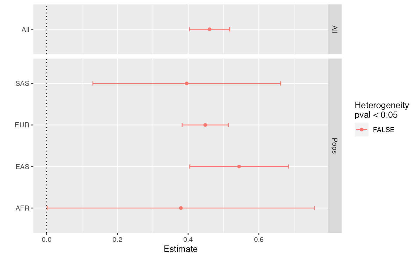

Evaluate instrument specificity. First using heterogeneity

x$instrument_heterogeneity(x$instrument_fema)
#> # A tibble: 6 × 9
#>   Reference   Replication      nsnp agreement     se      pval      I2      Q
#>   <chr>       <chr>           <int>     <dbl>  <dbl>     <dbl>   <dbl>  <dbl>
#> 1 ukb-b-19953 ukb-e-23104_CSA   377     0.683 0.0502 3.92e- 42 0.129    433. 
#> 2 ukb-b-19953 ukb-e-21001_AFR   377     0.526 0.0774 1.02e- 11 0.302    540. 
#> 3 ukb-b-19953 bbj-a-1           377     0.696 0.0238 1.58e-188 0.710   1301. 
#> 4 bbj-a-1     ukb-e-23104_CSA    61     0.836 0.0766 1.04e- 27 0.00233   61.1
#> 5 bbj-a-1     ukb-e-21001_AFR    61     0.747 0.128  5.42e-  9 0.261     82.5
#> 6 bbj-a-1     ukb-b-19953        61     0.866 0.0354 7.68e-132 0.908    661. 
#> # ℹ 1 more variable: Q_pval <dbl>

In this example, compared to above, the agreement regression slopes are closer to 1 for all pairs of ancestries.

x$estimate_instrument_specificity(x$instrument_fema, alpha = "bonferroni")
#> Checking ukb-e-23104_CSA against ukb-e-21001_AFR
#> Checking ukb-e-23104_CSA against ukb-b-19953
#> Checking ukb-e-23104_CSA against bbj-a-1
#> Checking ukb-e-21001_AFR against ukb-e-23104_CSA
#> Checking ukb-e-21001_AFR against ukb-b-19953
#> Checking ukb-e-21001_AFR against bbj-a-1
#> Checking ukb-b-19953 against ukb-e-23104_CSA
#> Checking ukb-b-19953 against ukb-e-21001_AFR
#> Checking ukb-b-19953 against bbj-a-1
#> Checking bbj-a-1 against ukb-e-23104_CSA
#> Checking bbj-a-1 against ukb-e-21001_AFR
#> Checking bbj-a-1 against ukb-b-19953
#>          discovery     replication nsnp  metric    datum       value
#> 1  ukb-e-21001_AFR ukb-e-23104_CSA    1 P-value Expected   0.9987782
#> 2  ukb-e-21001_AFR ukb-e-23104_CSA    1 P-value Observed   1.0000000
#> 3  ukb-e-21001_AFR ukb-e-23104_CSA    1    Sign Expected   0.9999995
#> 4  ukb-e-21001_AFR ukb-e-23104_CSA    1    Sign Observed   1.0000000
#> 5  ukb-e-21001_AFR     ukb-b-19953    1 P-value Expected   1.0000000
#> 6  ukb-e-21001_AFR     ukb-b-19953    1 P-value Observed   1.0000000
#> 7  ukb-e-21001_AFR     ukb-b-19953    1    Sign Expected   0.9999995
#> 8  ukb-e-21001_AFR     ukb-b-19953    1    Sign Observed   1.0000000
#> 9  ukb-e-21001_AFR         bbj-a-1    1 P-value Expected   1.0000000
#> 10 ukb-e-21001_AFR         bbj-a-1    1 P-value Observed   1.0000000
#> 11 ukb-e-21001_AFR         bbj-a-1    1    Sign Expected   0.9999995
#> 12 ukb-e-21001_AFR         bbj-a-1    1    Sign Observed   1.0000000
#> 13     ukb-b-19953 ukb-e-23104_CSA  377 P-value Expected   1.8062068
#> 14     ukb-b-19953 ukb-e-23104_CSA  377 P-value Observed   2.0000000
#> 15     ukb-b-19953 ukb-e-23104_CSA  377    Sign Expected 314.6226158
#> 16     ukb-b-19953 ukb-e-23104_CSA  377    Sign Observed 271.0000000
#> 17     ukb-b-19953 ukb-e-21001_AFR  377 P-value Expected   0.3238810
#> 18     ukb-b-19953 ukb-e-21001_AFR  377 P-value Observed   1.0000000
#> 19     ukb-b-19953 ukb-e-21001_AFR  377    Sign Expected 285.3702608
#> 20     ukb-b-19953 ukb-e-21001_AFR  377    Sign Observed 225.0000000
#> 21     ukb-b-19953         bbj-a-1  377 P-value Expected 127.5615021
#> 22     ukb-b-19953         bbj-a-1  377 P-value Observed  58.0000000
#> 23     ukb-b-19953         bbj-a-1  377    Sign Expected 372.6560995
#> 24     ukb-b-19953         bbj-a-1  377    Sign Observed 329.0000000
#> 25         bbj-a-1 ukb-e-23104_CSA   61 P-value Expected   1.5812878
#> 26         bbj-a-1 ukb-e-23104_CSA   61 P-value Observed   2.0000000
#> 27         bbj-a-1 ukb-e-23104_CSA   61    Sign Expected  55.5707081
#> 28         bbj-a-1 ukb-e-23104_CSA   61    Sign Observed  51.0000000
#> 29         bbj-a-1 ukb-e-21001_AFR   61 P-value Expected   0.2222185
#> 30         bbj-a-1 ukb-e-21001_AFR   61 P-value Observed   1.0000000
#> 31         bbj-a-1 ukb-e-21001_AFR   61    Sign Expected  50.7653607
#> 32         bbj-a-1 ukb-e-21001_AFR   61    Sign Observed  43.0000000
#> 33         bbj-a-1     ukb-b-19953   61 P-value Expected  60.5406720
#> 34         bbj-a-1     ukb-b-19953   61 P-value Observed  57.0000000
#> 35         bbj-a-1     ukb-b-19953   61    Sign Expected  60.9999028
#> 36         bbj-a-1     ukb-b-19953   61    Sign Observed  61.0000000
#>           pdiff
#> 1  1.000000e+00
#> 2  1.000000e+00
#> 3  1.000000e+00
#> 4  1.000000e+00
#> 5  1.000000e+00
#> 6  1.000000e+00
#> 7  1.000000e+00
#> 8  1.000000e+00
#> 9  1.000000e+00
#> 10 1.000000e+00
#> 11 1.000000e+00
#> 12 1.000000e+00
#> 13 7.031463e-01
#> 14 7.031463e-01
#> 15 2.038430e-08
#> 16 2.038430e-08
#> 17 2.767644e-01
#> 18 2.767644e-01
#> 19 6.677149e-12
#> 20 6.677149e-12
#> 21 1.087440e-15
#> 22 1.087440e-15
#> 23 3.515845e-34
#> 24 3.515845e-34
#> 25 6.729494e-01
#> 26 6.729494e-01
#> 27 6.573025e-02
#> 28 6.573025e-02
#> 29 1.995844e-01
#> 30 1.995844e-01
#> 31 1.478408e-02
#> 32 1.478408e-02
#> 33 1.191887e-03
#> 34 1.191887e-03
#> 35 1.000000e+00
#> 36 1.000000e+00
x$instrument_specificity$distinct %>% table
#> .
#> FALSE  TRUE 
#>  1148   169

Instruments with distinct equal to TRUE were expected to replicate, or to have the same sign, in another population but did not.

Evaluate similarity of pleiotropy across ancestry

Note: the term pleiotropy used here refers to ‘horizontal pleiotropy’, the influence of the SNP on the outcome not mediated through the exposure.

Here we will find pleiotropy outliers from the MR analysis, and then determine if the deviation of those outliers from the overall MR estimates is consistent across populations

x$pleiotropy()

Outliers are detected based on whether a SNP’s Wald ratio (in a particular population) is substantially different from the overall estimate. The overall estimate is the combined meta-analysis across all populations and all SNPs, unless that population’s overall MR estimate contributed substantially to heterogeneity. In that case, deviation is estimated based on the population’s specific MR estimate.

x$pleiotropy_outliers
#> # A tibble: 36 × 16
#>    SNP         pops    beta.x    se.x   beta.y    se.y   pval.x  pval.y       wr
#>    <chr>       <chr>    <dbl>   <dbl>    <dbl>   <dbl>    <dbl>   <dbl>    <dbl>
#>  1 10:1049422… SAS    0.0154  0.0176   3.00e-2 0.0546  1.90e- 1 2.91e-1  1.95e+0
#>  2 10:1049422… AFR    0.0732  0.0867  -1.10e-5 0.385   1.99e- 1 5.00e-1 -1.50e-4
#>  3 10:1049422… EUR    0.0238  0.00370 -7.70e-2 0.0144  6.14e-11 4.69e-8 -3.24e+0
#>  4 10:1049422… EAS    0.0253  0.00423 -2.79e-2 0.0177  1.12e- 9 5.73e-2 -1.10e+0
#>  5 11:1331520… SAS    0.00115 0.0145  -4.07e-2 0.0453  4.68e- 1 1.84e-1 -3.55e+1
#>  6 11:1331520… AFR   -0.102   0.0381  -2.18e-2 0.168   3.81e- 3 4.49e-1  2.14e-1
#>  7 11:1331520… EUR    0.0164  0.00200  4.00e-2 0.00974 1.15e-16 2.00e-5  2.44e+0
#>  8 11:1331520… EAS    0.0103  0.00451  8.29e-3 0.0189  1.13e- 2 3.30e-1  8.06e-1
#>  9 11:1169473… SAS   -0.00940 0.0267  -7.18e-2 0.0830  3.62e- 1 1.93e-1  7.64e+0
#> 10 11:1169473… AFR   -0.0268  0.0327   1.15e-1 0.144   2.06e- 1 2.12e-1 -4.28e+0
#> # ℹ 26 more rows
#> # ℹ 7 more variables: wr.se <dbl>, biv <dbl>, biv.se <dbl>, dif <dbl>,
#> #   dif.se <dbl>, Qj <dbl>, Qjpval <dbl>

For outliers from a population, are other populations showing similar deviation to the outlier discovery population? e.g. look at whether the sign is the same for outliers discovered in Europeans:

x$pleiotropy_agreement %>% as.data.frame %>% subset(disc == "EUR" & metric=="Sign")
#>    disc rep nsnp metric    datum    value       pdiff
#> 15  EUR SAS    7   Sign Expected 5.410300 0.051335225
#> 16  EUR SAS    7   Sign Observed 3.000000 0.051335225
#> 19  EUR AFR    7   Sign Expected 4.979110 0.111858226
#> 20  EUR AFR    7   Sign Observed 3.000000 0.111858226
#> 23  EUR EAS    7   Sign Expected 6.553344 0.007480742
#> 24  EUR EAS    7   Sign Observed 4.000000 0.007480742

Look at the overall relationship of outlier deviations across populations

x$plot_pleiotropy()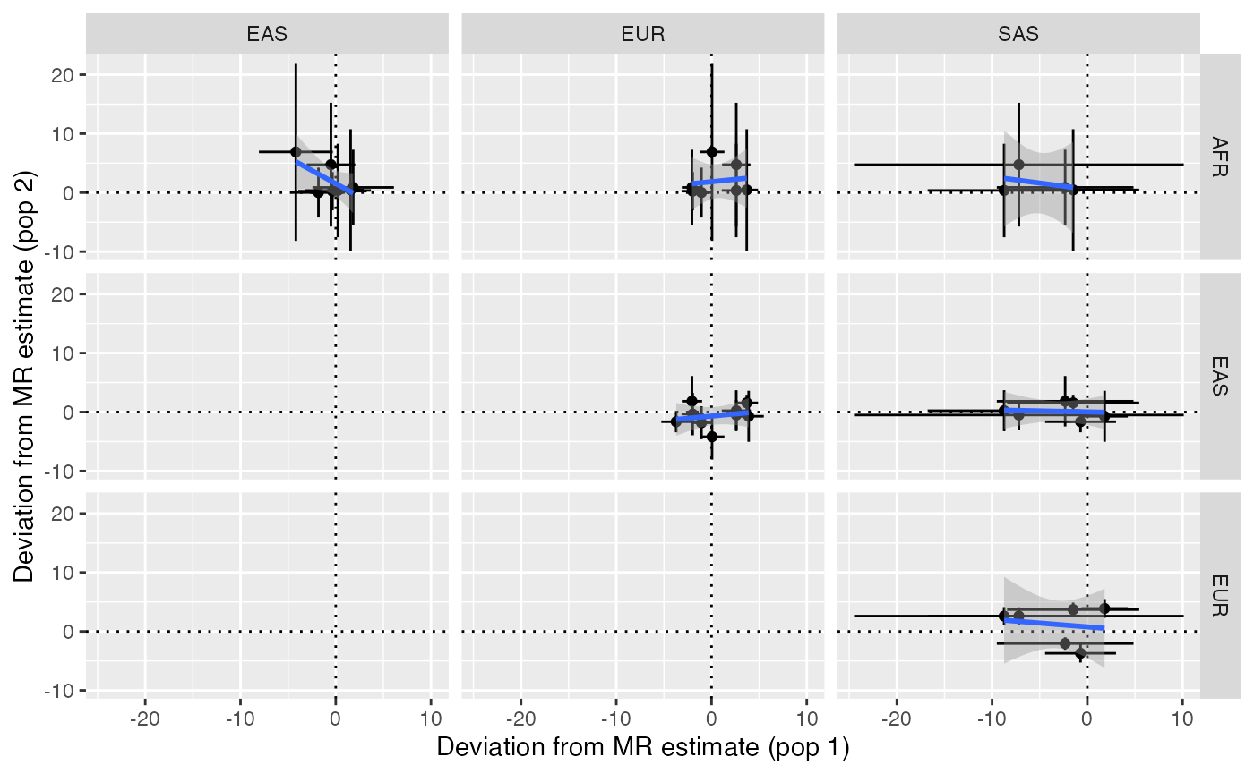

Identify any variants that showed substantial differences in pleiotropy deviations across populations. Note that sometimes the pleiotropy deviation estimate is unstable due to the SNP-exposure association being very small. Unstable estimates are attempted to be removed automatically from the heterogeneity analysis

x$plot_pleiotropy_heterogeneity(pthresh=0.05)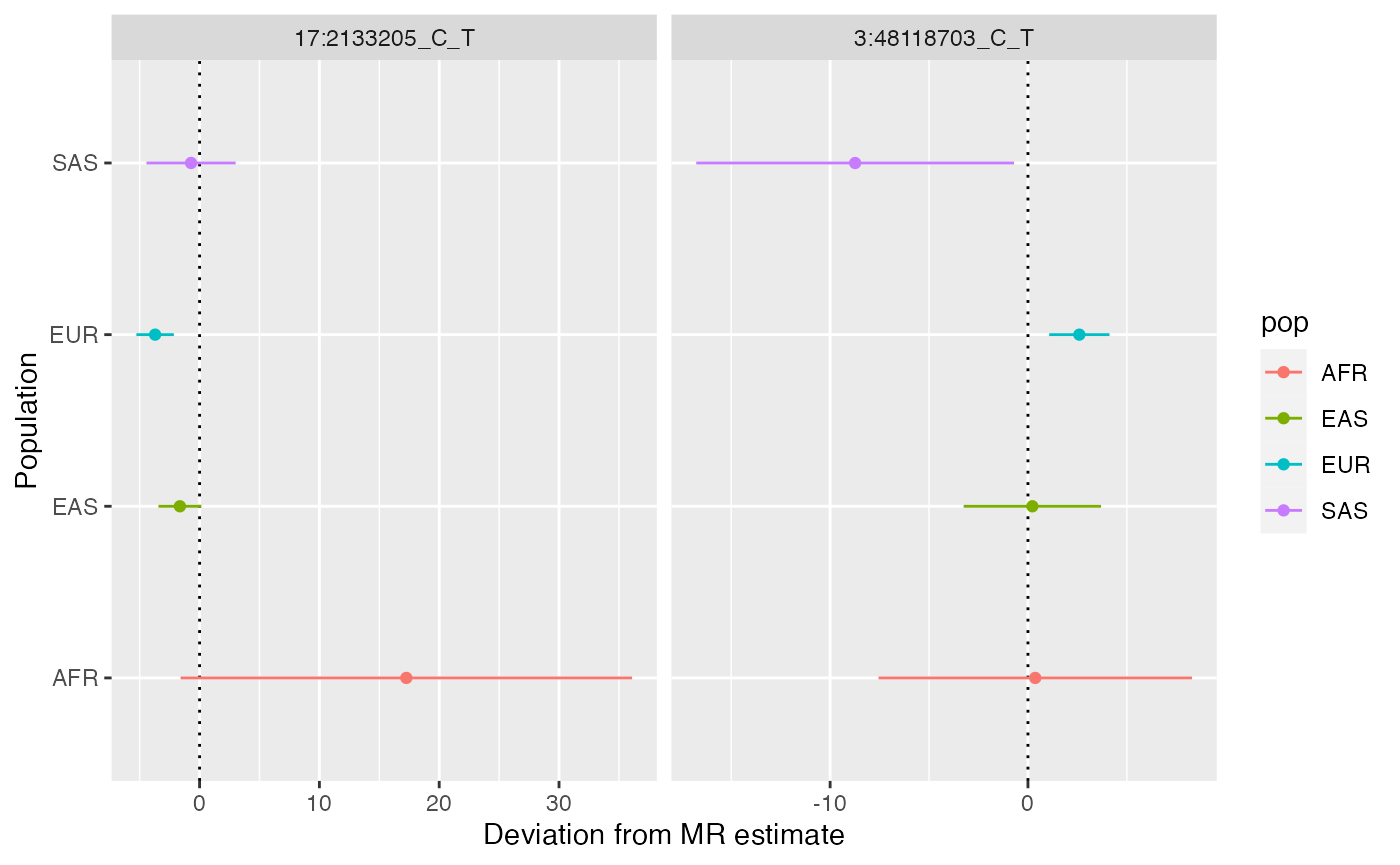

In this example two SNPs show evidence of differences in pleiotropy deviation across populations. For 17:2133205_C_T this is driven by the very imprecise estimate in AFR, and for 3:48118703_C_T by the SAS and EUR estimates deviating in opposite directions. Plot everything by relaxing the threshold

x$plot_pleiotropy_heterogeneity(pthresh=1)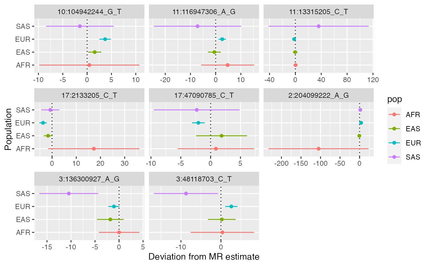

MR GxE

The MR GxE model aims to estimate the horizontal pleiotropic effect of a SNP. This is achieved by estimating its effect on the outcome in a subset of the data where the SNP is not expected to have an association (the zero relevance group). The cross-ancestry MR analysis can attempt to make use of this approach by identifying variants that exhibit heterogeneity in the instrument-exposure association across ancestries. Those instruments can then be used to estimate the pleiotropic association by evaluating their effect on the outcome across populations showing differential SNP-exposure associations.

First identify examples of heterogeneity amongst instrument-exposure associations

x$estimate_instrument_heterogeneity_per_variant()
#> # A tibble: 381 × 5
#>    SNP                Qdf      Q     Qpval    Qfdr
#>    <chr>            <dbl>  <dbl>     <dbl>   <dbl>
#>  1 10:104942244_G_T     3  0.650 0.885     0.926  
#>  2 10:118650996_C_T     3 17.7   0.000502  0.00710
#>  3 10:132953074_C_T     3 22.3   0.0000556 0.00125
#>  4 10:134007008_A_C     3  8.12  0.0436    0.173  
#>  5 10:16750129_G_T      3  0.510 0.917     0.941  
#>  6 10:18573654_A_G      3  6.63  0.0847    0.238  
#>  7 10:21830104_A_G      3  3.19  0.363     0.574  
#>  8 10:33955430_C_T      3 13.5   0.00375   0.0275 
#>  9 10:53673286_A_G      3  4.26  0.235     0.457  
#> 10 10:61842645_C_T      3  6.16  0.104     0.264  
#> # ℹ 371 more rows
x$instrument_heterogeneity_per_variant %>% dplyr::filter(Qfdr < 0.05)
#> # A tibble: 65 × 5
#>    SNP                Qdf     Q      Qpval     Qfdr
#>    <chr>            <dbl> <dbl>      <dbl>    <dbl>
#>  1 10:118650996_C_T     3  17.7 0.000502   0.00710 
#>  2 10:132953074_C_T     3  22.3 0.0000556  0.00125 
#>  3 10:33955430_C_T      3  13.5 0.00375    0.0275  
#>  4 10:99772885_A_G      3  18.8 0.000298   0.00494 
#>  5 11:130795698_G_T     3  14.5 0.00232    0.0213  
#>  6 11:13315205_C_T      3  11.9 0.00786    0.0464  
#>  7 11:2858440_A_G       3  29.5 0.00000179 0.000170
#>  8 11:43648368_G_T      3  12.4 0.00627    0.0412  
#>  9 11:65640906_C_T      3  24.2 0.0000222  0.000732
#> 10 12:103658096_A_G     3  13.2 0.00428    0.0301  
#> # ℹ 55 more rows

Next perform MR GxE (may take a couple of minutes while bootstrapping standard errors)

set.seed(1234)
x$mrgxe()
#> # A tibble: 65 × 9
#>    SNP                     a      b   a_se  b_se a_pval b_pval   a_mean  b_mean
#>    <chr>               <dbl>  <dbl>  <dbl> <dbl>  <dbl>  <dbl>    <dbl>   <dbl>
#>  1 10:118650996_C_T  0.0450   2.14  0.0253  1.60 0.0377 0.0903  0.0459   2.10  
#>  2 10:132953074_C_T -0.0399   3.84  0.0346  3.34 0.125  0.125  -0.0457   1.84  
#>  3 10:33955430_C_T   0.00610 -0.195 0.0419  1.85 0.442  0.458   0.00721 -0.137 
#>  4 10:99772885_A_G  -0.0195  -1.48  0.0277  1.89 0.241  0.218  -0.0201  -1.32  
#>  5 11:130795698_G_T -0.0110   2.17  0.0315  1.78 0.363  0.111  -0.00974  2.12  
#>  6 11:13315205_C_T   0.00168  0.283 0.0227  1.63 0.471  0.431   0.00383  0.425 
#>  7 11:2858440_A_G   -0.0848   1.42  0.119   3.07 0.238  0.322  -0.0461  -0.0876
#>  8 11:43648368_G_T   0.0164   1.53  0.0302  1.56 0.293  0.163   0.0163   0.969 
#>  9 11:65640906_C_T   0.0157  -1.70  0.0307  1.80 0.304  0.172   0.0121  -1.09  
#> 10 12:103658096_A_G  0.0639  -2.25  0.0466  2.23 0.0850 0.157   0.0554  -1.85  
#> # ℹ 55 more rows

This is the distribution of the estimate of the pleiotropic effect of each SNP that showed heterogeneity

x$mrgxe_plot()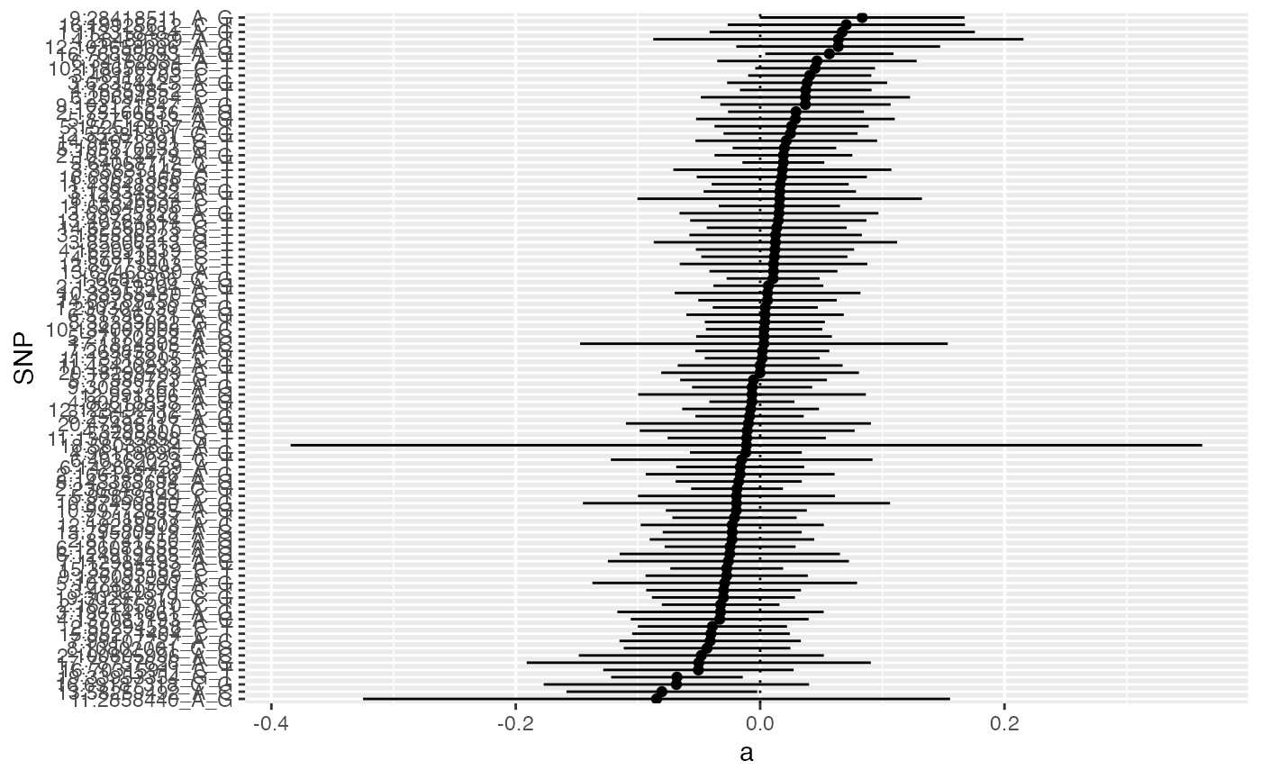

Any SNPs with evidence of a pleiotropic effect?

x$mrgxe_res %>% dplyr::filter(p.adjust(a_pval, "fdr") < 0.05)
#> # A tibble: 0 × 9
#> # ℹ 9 variables: SNP <chr>, a <dbl>, b <dbl>, a_se <dbl>, b_se <dbl>,
#> #   a_pval <dbl>, b_pval <dbl>, a_mean <dbl>, b_mean <dbl>

In this example none of the pleiotropy estimates pass FDR < 0.05. It’s worth always checking if any SNPs look credible e.g. this plots the SNP-exposure against SNP-outcome associations for the SNPs with nominal p < 0.05 (by default mrgxe_plot_variant() plots the SNPs with FDR < 0.05). You’d expect to see a slope reflecting the causal effect estimate with the intercept reflecting the pleiotropic association.

x$mrgxe_plot_variant(subset(x$mrgxe_res, a_pval < 0.05)$SNP)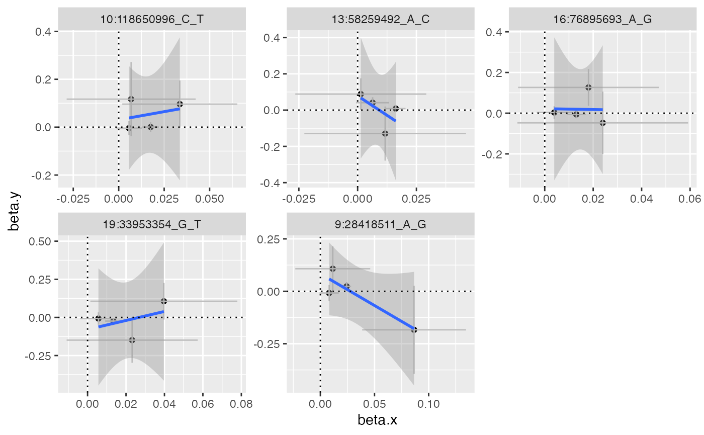

In this case the associations are very noisy, and it would be difficult to justify that they show convincing evidence of the pleiotropy estimate.

Saving and loading data

It can be useful to import data from one CAMERA object to another, because for example you may have all your data, but the CAMERA class has been updated, and you want to initialise a new class and import all the old data into the new class.

Save CAMERA objects as RDS files e.g.

saveRDS(x, file="example-CAMERA.rds")

And load them like this:

x <- readRDS(file="example-CAMERA.rds")

You can import data from one CAMERA object to another like this:

x_new <- CAMERA$new()
x_new$import(x)

Overview of methods

The analysis functions in CAMeRa are methods of the CAMERA class, so they are called as x$method() and are documented together on the CAMERA reference page (or ?CAMERA). The methods used in this vignette, in the order they are used, are:

Step	Method	Results
Check phenotype scales across ancestries	`check_phenotypes()`	Printed table
Extract instruments	`extract_instruments()`	`x$instrument_raw`
Instrument heterogeneity across populations	`instrument_heterogeneity()`	Returned table
Instrument specificity across populations	`estimate_instrument_specificity()`	`x$instrument_specificity_summary`, `x$instrument_specificity`
Extract outcome data	`make_outcome_data()`	`x$instrument_outcome`
Harmonise exposure and outcome data	`harmonise()`	`x$harmonised_dat`
MR within and across populations	`cross_estimate()`	`x$mrres`
Plot MR estimates	`plot_cross_estimate()`	Plot
Extract regions around instruments	`extract_instrument_regions()`	`x$instrument_regions`
Select regional instruments by meta analysis	`fema_regional_instruments()`	`x$instrument_fema`, `x$instrument_fema_regions`
Plot a region	`plot_regional_instruments()`	Plot
Pleiotropy across ancestries	`pleiotropy()`	`x$pleiotropy_outliers`, `x$pleiotropy_Q_outliers`, `x$pleiotropy_agreement`
Plot pleiotropy	`plot_pleiotropy()`, `plot_pleiotropy_heterogeneity()`	Plots
Per variant instrument-exposure heterogeneity	`estimate_instrument_heterogeneity_per_variant()`	`x$instrument_heterogeneity_per_variant`
MR GxE	`mrgxe()`	`x$mrgxe_res`
Plot MR GxE results	`mrgxe_plot()`, `mrgxe_plot_variant()`	Plots