Variance estimators

Data generating model

\[ y_i = \alpha + \beta_{1,j}G_{ij} + z_i + v_i + e_i \]

where \(\alpha\) is an intercept term, \(\beta_{1,j}\) is the additive effect of SNP $j$, \(G_{i,j}\) is the genotype value for individual \(i\) at SNP $j$, \(z_i\) is the remaining polygenic risk

\[ z_i \sim N(0, \sigma^2_{g} - 2p_j(1-p_j)\beta_{1,j}^2) \]

\(v_i\) is the SNP’s influence on dispersion where

\[ v_i \sim N(0, \beta_{2,j}G_{i,j}) \]

and \(e_i\) is the residual variance

\[ e_i \sim N(0, 1 - \sigma^2_g - \sigma^2_v) \]

To estimate dispersion effects amongst unrelateds use the deviation regression model (DRM) from Marderstein et al 2021 AJHG (https://doi.org/10.1016/j.ajhg.2020.11.016).

To estimate variance heterogeneity effects using MZs, simply

\[ |y_{i,A} - y_{i,B}| = \hat{\beta}_{2,j}G_{i,j} + \epsilon_i \]

where A and B represent the individuals in the MZ pair.

To estimate variance heterogeneity effects using siblings, it is identical to the MZ method but restricted to sibling pairs who have identity by state value of 2 (i.e. share the same genotype value at the SNP being tested).

Simulations

library(dplyr)

Attaching package: 'dplyr'

The following objects are masked from 'package:stats':

    filter, lag

The following objects are masked from 'package:base':

    intersect, setdiff, setequal, union

library(ggplot2)

Method for simulating dispersion effects in unrelated individuals

sim_pop <- function(n, beta1, beta2, af, h2)
{
  g <- rbinom(n, 2, af)
  prs <- g * beta1
  vg <- rnorm(n, 0, h2)
  v <- rnorm(n, 0, beta2 * g)
  ve <- rnorm(n, 0, sqrt(1 - var(vg) - var(v) - var(prs)))
  y <- prs + v + vg + ve
  return(tibble(
    g, y
  ))
}
a <- sim_pop(100000, 0.1, 0.5, 0.3, 0.1)
var(a)

           g          y
g 0.41881431 0.04145241
y 0.04145241 1.00183156

Method for simulating dispersion effects in monozogytic twins

sim_mz <- function(n, beta1, beta2, af, h2)
{
  g <- rbinom(n, 2, af)
  prs <- g * beta1
  vg <- rnorm(n, 0, h2)
  v1 <- rnorm(n, 0, beta2 * g)
  ve1 <- rnorm(n, 0, sqrt(1 - var(vg) - var(v1) - var(prs)))
  y1 <- prs + v1 + vg + ve1
  v2 <- rnorm(n, 0, beta2 * g)
  ve2 <- rnorm(n, 0, sqrt(1 - var(vg) - var(v2) - var(prs)))
  y2 <- prs + v2 + vg + ve2
  return(tibble(
    g, y1, y2
  ))
}
a <- sim_mz(100000, 0.1, 0.5, 0.3, 0.1)
var(a)

            g         y1         y2
g  0.41789069 0.04179887 0.04360385
y1 0.04179887 1.00074619 0.01158774
y2 0.04360385 0.01158774 0.99856453

See what dispersion looks like from this simulation

a %>%
  ggplot(., aes(x=as.factor(g), y=y1)) +
  geom_boxplot()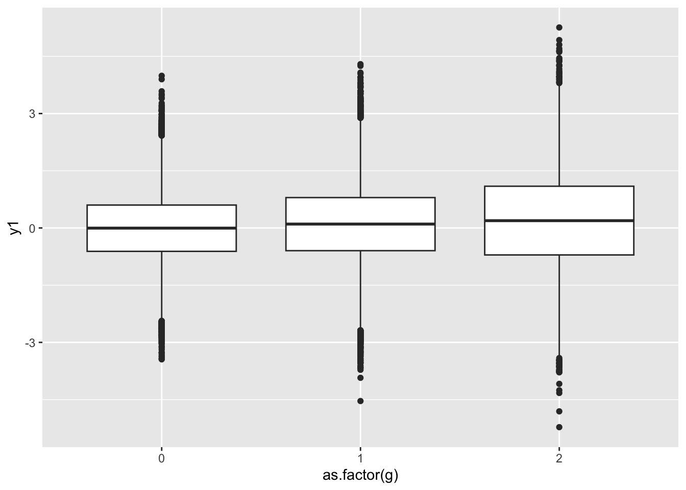

Summarise the dispersion. Note - how would you scale it to the MZ pair mean?

a <- sim_mz(100000, 0.1, 0.5, 0.3, 0.8)
a %>% 
  group_by(g) %>% 
  summarise(
    m=mean(y1), 
    v=var(y1), 
    mzv=mean(abs(y1-y2))
  )

# A tibble: 3 × 4
      g        m     v   mzv
  <int>    <dbl> <dbl> <dbl>
1     0 -0.00271 0.795 0.456
2     1  0.102   1.06  0.724
3     2  0.211   1.83  1.21 

Method for testing unrelateds using DRM

test_drm <- function(g, y)
{
  y.i <- tapply(y, g, median, na.rm=T)  
  z.ij <- abs(y - y.i[g+1])
  summary(lm(z.ij ~ g))$coef %>%
    as_tibble() %>%
    slice(2) %>%
    mutate(method="drm")
}
test_drm(a$g, a$y1)

# A tibble: 1 × 5
  Estimate `Std. Error` `t value` `Pr(>|t|)` method
     <dbl>        <dbl>     <dbl>      <dbl> <chr> 
1    0.152      0.00295      51.6          0 drm   

Method for testing using MZs

test_mz <- function(g, y1, y2)
{
  yd1 <- abs(y1-y2)
  r1 <- summary(lm(yd1 ~ g))$coef %>%
    as_tibble() %>%
    slice(2) %>%
    mutate(method="mzdiff")
  r1
}

test_mz(a$g, a$y1, a$y2)

# A tibble: 1 × 5
  Estimate `Std. Error` `t value` `Pr(>|t|)` method
     <dbl>        <dbl>     <dbl>      <dbl> <chr> 
1    0.332      0.00249      133.          0 mzdiff

Power simulations

A trait with high heritability will have vQTL (dispersion) effects that are relatively large in MZs, but heritability shouldn’t have a major part to play in unrelateds for estimating vQTL effects.

Start with simulations where population is compared against mz and n pop = n mz pairs.

param <- expand.grid(
  beta1 = 0,
  beta2 = seq(0, 0.5, by=0.01),
  h2 = c(0.1, 0.9),
  af = 0.3,
  n = 10000
)
dim(param)

[1] 102   5

res1 <- lapply(1:nrow(param), function(i)
  {
  a <- do.call(sim_mz, param[i,])
  if(any(is.na(a$y1)) | any(is.na(a$y2)))
  {
    return(NULL)
  }
  bind_rows(
    test_mz(a$g, a$y1, a$y2),
    test_drm(a$g, a$y1)
  ) %>%
    bind_cols(., param[i,])
}) %>%
  bind_rows()

res1 %>% filter(n==10000) %>%
ggplot(., aes(x=beta2, y=-log10(`Pr(>|t|)`))) +
  geom_line(aes(colour=method)) +
  facet_grid(. ~ h2)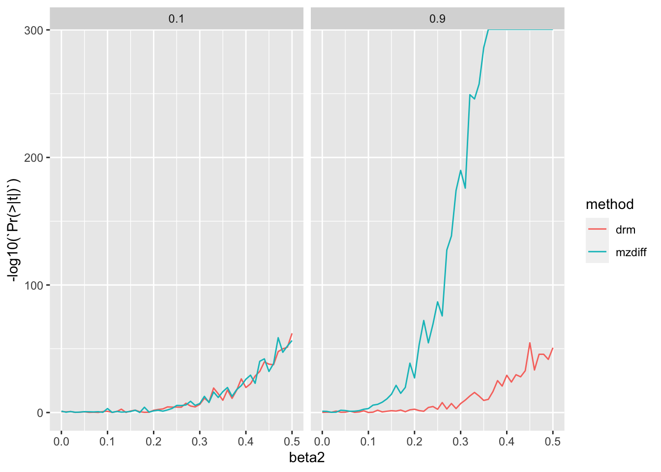

They are comparable at low heritability but as heritability increases, MZ method has a distinct advantage.

Now compare with more realistic sample sizes, 10k mz pairs vs 500k unrelateds

param <- expand.grid(
  beta1 = 0,
  beta2 = seq(0, 0.5, by=0.01),
  h2 = c(0.1, 0.9),
  af = 0.32
)
dim(param)

[1] 102   4

res2 <- lapply(1:nrow(param), function(i)
  {
  a1 <- do.call(sim_mz, param[i,] %>% mutate(n=10000))
  a2 <- do.call(sim_mz, param[i,] %>% mutate(n=500000))
  if(any(is.na(a1$y1)) | any(is.na(a1$y2)) | any(is.na(a2$y1)) | any(is.na(a2$y2)))
  {
    return(NULL)
  }
  bind_rows(
    test_mz(a1$g, a1$y1, a1$y2),
    test_drm(a2$g, a2$y1)
  ) %>%
    bind_cols(., param[i,])
}) %>%
  bind_rows()

Warning in sqrt(1 - var(vg) - var(v1) - var(prs)): NaNs produced

Warning in rnorm(n, 0, sqrt(1 - var(vg) - var(v1) - var(prs))): NAs produced

Warning in sqrt(1 - var(vg) - var(v2) - var(prs)): NaNs produced

Warning in rnorm(n, 0, sqrt(1 - var(vg) - var(v2) - var(prs))): NAs produced

Warning in sqrt(1 - var(vg) - var(v1) - var(prs)): NaNs produced

Warning in rnorm(n, 0, sqrt(1 - var(vg) - var(v1) - var(prs))): NAs produced

Warning in sqrt(1 - var(vg) - var(v2) - var(prs)): NaNs produced

Warning in rnorm(n, 0, sqrt(1 - var(vg) - var(v2) - var(prs))): NAs produced

Warning in sqrt(1 - var(vg) - var(v1) - var(prs)): NaNs produced

Warning in rnorm(n, 0, sqrt(1 - var(vg) - var(v1) - var(prs))): NAs produced

Warning in sqrt(1 - var(vg) - var(v2) - var(prs)): NaNs produced

Warning in rnorm(n, 0, sqrt(1 - var(vg) - var(v2) - var(prs))): NAs produced

Warning in sqrt(1 - var(vg) - var(v1) - var(prs)): NaNs produced

Warning in rnorm(n, 0, sqrt(1 - var(vg) - var(v1) - var(prs))): NAs produced

Warning in sqrt(1 - var(vg) - var(v2) - var(prs)): NaNs produced

Warning in rnorm(n, 0, sqrt(1 - var(vg) - var(v2) - var(prs))): NAs produced

Warning in sqrt(1 - var(vg) - var(v1) - var(prs)): NaNs produced

Warning in rnorm(n, 0, sqrt(1 - var(vg) - var(v1) - var(prs))): NAs produced

Warning in sqrt(1 - var(vg) - var(v2) - var(prs)): NaNs produced

Warning in rnorm(n, 0, sqrt(1 - var(vg) - var(v2) - var(prs))): NAs produced

ggplot(res2, aes(x=beta2, y=-log10(`Pr(>|t|)`))) +
  geom_line(aes(colour=method)) +
  facet_grid(. ~ h2)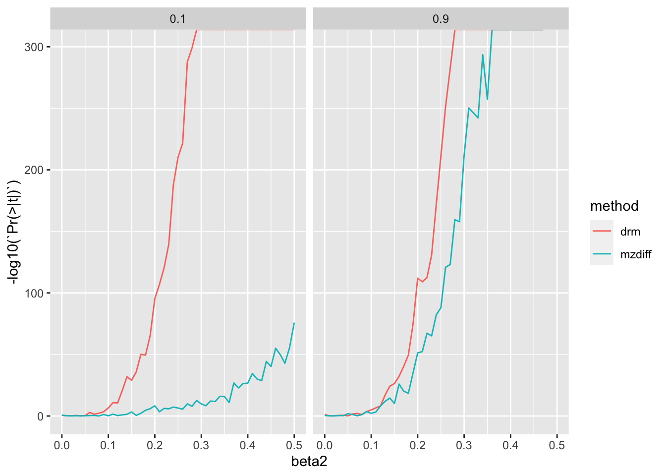

It looks like you’d just be better off with estimation in populations.

Type 1 error

param <- expand.grid(
  beta1 = seq(0, 0.5, by=0.002),
  beta2 = 0,
  h2 = c(0.1, 0.9),
  af = 0.32
)
dim(param)

[1] 502   4

res3 <- lapply(1:nrow(param), function(i)
  {
  a1 <- do.call(sim_mz, param[i,] %>% mutate(n=10000))
  a2 <- do.call(sim_mz, param[i,] %>% mutate(n=500000))
  if(any(is.na(a1$y1)) | any(is.na(a1$y2)) | any(is.na(a2$y1)) | any(is.na(a2$y2)))
  {
    return(NULL)
  }
  bind_rows(
    test_mz(a1$g, a1$y1, a1$y2),
    test_drm(a2$g, a2$y1)
  ) %>%
    bind_cols(., param[i,])
}) %>%
  bind_rows()

Plot type 1 error

ggplot(res3, aes(x=beta1, y=-log10(`Pr(>|t|)`))) +
  geom_line(aes(colour=method)) +
  facet_grid(. ~ h2)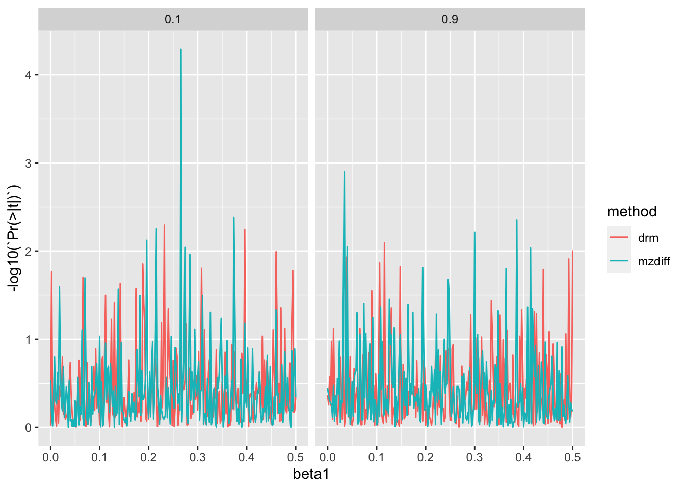

Type 1 error and number of false positives after multiple testing correction

res3 %>% 
  mutate(fdr=p.adjust(`Pr(>|t|)`, "fdr")) %>%
  group_by(method, h2) %>%
  summarise(
    t1 = sum(`Pr(>|t|)` < 0.05, na.rm=T)/sum(!is.na(`Pr(>|t|)`)),
    nfdr = sum(fdr < 0.05)/sum(!is.na(`Pr(>|t|)`))
  )

`summarise()` has grouped output by 'method'. You can override using the
`.groups` argument.

# A tibble: 4 × 4
# Groups:   method [2]
  method    h2     t1  nfdr
  <chr>  <dbl>  <dbl> <dbl>
1 drm      0.1 0.0637     0
2 drm      0.9 0.0478     0
3 mzdiff   0.1 0.0558     0
4 mzdiff   0.9 0.0757     0

Under normal distribution type-1 error rate is well controlled.

Simulations using siblings

Generate a set of sib pairs with the following specification

• Have PRS such that IBD ~ N(0.5, sqrt(0.037))

• h2 specified

• ce specified (shared variance between sibs

• one SNP has a mean and variance effect

• scaled phenotypes ~ N(0, 1)

sim_sibs <- function(af, nfam, beta1, beta2, h2, c2)
{
  # Choose number of SNPs to be expected number of recombination events
  # in order to give appropriate distribution of IBD
    nsnp <- 87
    af <- rep(af, nsnp)
    dads <- matrix(0, nfam, nsnp)
    mums <- matrix(0, nfam, nsnp)
    sibs1 <- matrix(0, nfam, nsnp)
    sibs2 <- matrix(0, nfam, nsnp)
    ibd <- matrix(0, nfam, nsnp)
    ibs <- matrix(0, nfam, nsnp)
    for(i in 1:nsnp)
    {
        dad1 <- rbinom(nfam, 1, af[i]) + 1
        dad2 <- (rbinom(nfam, 1, af[i]) + 1) * -1
        mum1 <- rbinom(nfam, 1, af[i]) + 1
        mum2 <- (rbinom(nfam, 1, af[i]) + 1) * -1

        dadindex <- sample(c(TRUE, FALSE), nfam, replace=TRUE)
        dadh <- rep(NA, nfam)
        dadh[dadindex] <- dad1[dadindex]
        dadh[!dadindex] <- dad2[!dadindex]

        mumindex <- sample(c(TRUE, FALSE), nfam, replace=TRUE)
        mumh <- rep(NA, nfam)
        mumh[mumindex] <- mum1[mumindex]
        mumh[!mumindex] <- mum2[!mumindex]

        sib1 <- cbind(dadh, mumh)

        dadindex <- sample(c(TRUE, FALSE), nfam, replace=TRUE)
        dadh <- rep(NA, nfam)
        dadh[dadindex] <- dad1[dadindex]
        dadh[!dadindex] <- dad2[!dadindex]

        mumindex <- sample(c(TRUE, FALSE), nfam, replace=TRUE)
        mumh <- rep(NA, nfam)
        mumh[mumindex] <- mum1[mumindex]
        mumh[!mumindex] <- mum2[!mumindex]

        sib2 <- cbind(dadh, mumh)

        ibd[,i] <- (as.numeric(sib1[,1] == sib2[,1]) + as.numeric(sib1[,2] == sib2[,2])) / 2

        sibs1[,i] <- rowSums(abs(sib1) - 1)
        sibs2[,i] <- rowSums(abs(sib2) - 1)
        dads[,i] <- dad1 - 1 + abs(dad2) - 1
        mums[,i] <- mum1 - 1 + abs(mum2) - 1

        # l[[i]] <- (sum(sib1[,1] == sib2[,1]) / nsnp + sum(sib1[,2] == sib2[,2]) / nsnp) / 2

    }
    n <- nfam
    # Make phenotypes
    ce <- rnorm(n, 0, sqrt(c2))
    v1 <- rnorm(n, 0, beta2 * sibs1[,1])
    v2 <- rnorm(n, 0, beta2 * sibs2[,1])
    e1 <- rnorm(n, 0, sqrt(1 - h2 - c2 - var(v1)))
    e2 <- rnorm(n, 0, sqrt(1 - h2 - c2 - var(v2)))
    b <- rnorm(nsnp-1, 0, 1)
    h2_1 <- beta1^2 * af[1] * (1-af[1]) * 2
    h2_res <- h2 - h2_1
    prs1 <- scale(sibs1[,-1] %*% b) * sqrt(h2_res)
    prs2 <- scale(sibs2[,-1] %*% b) * sqrt(h2_res)
    y1 <- sibs1[,1] * beta1 + prs1 + v1 + ce + e1
    y2 <- sibs2[,1] * beta1 + prs2 + v2 + ce + e2
    return(tibble(
      ibd = rowMeans(ibd),
      g1 = sibs1[,1],
      g2 = sibs2[,1],
      prs1,
      prs2,
      y1, 
      y2
    ))
}

Notes

• In this model if the allele frequency is higher, then the genotype class with the larger variance is more common, which means that effect alleles are not reflexive in terms of variances

• I think this use with siblings may have problems due to LD. If there is incomplete LD with another causal variant elsewhere close by then the mean effect of that causal variant will contribute to the variance effect estimated at the variant

fam <- sim_sibs(0.3, 10000, 0.1, 0.4, 0.6, 0.1)
cor(fam) %>% round(4)

         ibd      g1     g2    prs1    prs2     y1     y2
ibd   1.0000 -0.0020 0.0068 -0.0063 -0.0045 0.0054 0.0077
g1   -0.0020  1.0000 0.5061  0.0085  0.0212 0.0649 0.0551
g2    0.0068  0.5061 1.0000  0.0089  0.0076 0.0329 0.0665
prs1 -0.0063  0.0085 0.0089  1.0000  0.4877 0.7760 0.3816
prs2 -0.0045  0.0212 0.0076  0.4877  1.0000 0.3818 0.7721
y1    0.0054  0.0649 0.0329  0.7760  0.3818 1.0000 0.4011
y2    0.0077  0.0551 0.0665  0.3816  0.7721 0.4011 1.0000

Now how to estimate variance effect? At a locus restrict to sib pairs who are IBD = 1

fam <- sim_sibs(af=0.5, nfam=40000, beta1=0.1, beta2=0.2, h2=0.3, c2=0.1)
fam

# A tibble: 40,000 × 7
     ibd    g1    g2 prs1[,1] prs2[,1]  y1[,1] y2[,1]
   <dbl> <dbl> <dbl>    <dbl>    <dbl>   <dbl>  <dbl>
 1 0.477     1     1 -0.333      0.360 -0.244   0.210
 2 0.437     2     2 -0.376     -0.516 -0.455   0.164
 3 0.511     1     1  0.0654    -0.613  0.247  -1.47 
 4 0.523     2     1  0.652      0.371  1.14    0.728
 5 0.506     0     0 -0.0106     0.456  0.0296  0.410
 6 0.483     1     2  0.0979     0.391  1.84    1.66 
 7 0.471     1     2  0.0902     0.495  0.0733 -0.518
 8 0.460     1     1 -0.451     -0.160 -0.941   0.344
 9 0.511     1     0  0.734      0.532  1.73    0.803
10 0.477     1     0  0.00962   -0.546  1.15   -0.801
# … with 39,990 more rows

Test for variance QTL

fam <- sim_sibs(af=0.5, nfam=40000, beta1=0.1, beta2=0.2, h2=0.01, c2=0.01)
f1 <- subset(fam, g1==g2)
test_mz(f1$g1, f1$y1, f1$y2)

# A tibble: 1 × 5
  Estimate `Std. Error` `t value` `Pr(>|t|)` method
     <dbl>        <dbl>     <dbl>      <dbl> <chr> 
1   0.0535      0.00795      6.73   1.78e-11 mzdiff

Power sims

param <- expand.grid(
  beta1 = 0,
  beta2 = seq(0, 0.5, by=0.01),
  c2 = c(0),
  h2 = c(0.1, 0.5),
  af = c(0.5)
)
dim(param)

[1] 102   5

res4 <- lapply(1:nrow(param), function(i)
  {
  a1 <- do.call(sim_sibs, param[i,] %>% mutate(nfam=22000))
  a2 <- do.call(sim_pop, param[i,] %>% select(-c(c2)) %>% mutate(n=500000))
  if(any(is.na(a1$y1)) | any(is.na(a1$y2)) | any(is.na(a2$y)))
  {
    return(NULL)
  }
  bind_rows(
    a1 %>% filter(g1==g2) %>% select(g=g1, y1, y2) %>% do.call(test_mz, .),
    do.call(test_drm, a2)
  ) %>%
    bind_cols(., param[i,])
}) %>%
  bind_rows()

res4 %>% mutate(sharing=c2+h2) %>% filter(beta1==0) %>%
  ggplot(., aes(x=beta2, y=-log10(`Pr(>|t|)`))) +
  geom_line(aes(colour=method, groups=af)) +
  facet_grid(. ~ sharing)

Warning in geom_line(aes(colour = method, groups = af)): Ignoring unknown
aesthetics: groups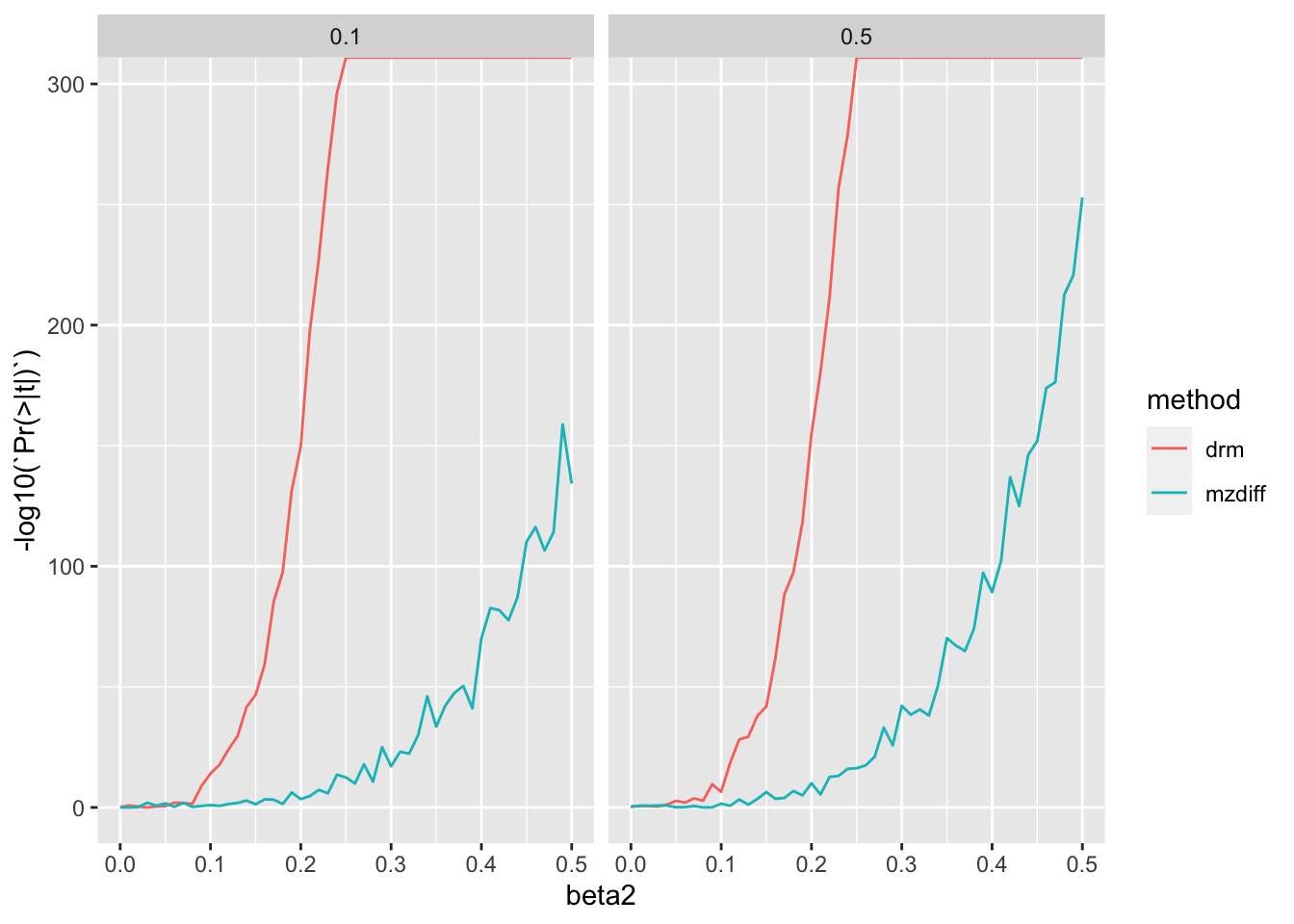

Similar to MZ method - quite a substantial benefit from leveraging large sample sizes of unrelateds compared to using siblings.